Translational States

Shaun Williams, PhD

The Free-Particle

• We are now going to tackle the simplest quantum mechanical system
• The system is a free-particle where "free" means that there are no forces acting on the particle
• Since a force is produced by a change in the potential energy, the potential energy must be constant if there is no force
• This constant can be taken to be zero because energy is relative not absolute

The Schrödinger Equation for the Free Particle

• Let's first go back to basics $$ \hat{\mathcal{H}}\psi=E\psi $$ $$ \hat{\mathcal{H}}=\hat{T}+\hat{V} $$
• We know that there is no potential energy for a free-particle and we know the one-dimensional kinetic energy operator $$ \hat{V}=V=0 \text{ and } \hat{T}=-\frac{\hbar^2}{2m} \frac{d^2}{dx^2} $$
• This gives us the Schrödinger equation for a free particle $$ \begin{equation} -\frac{\hbar^2}{2m}\frac{d^2 \psi(x)}{dx^2} = E\psi(x) \label{eq:5.1.5} \end{equation} $$

Solving the Free Particle Schrödinger

• A major problem in quantum mechanics is finding solutions to differential equations
• Differential equations keep arising because the operator for kinetic energy includes a second derivative
• We have already encountered this equation in the previous chapter
• This time, let's solve this equation by using some algebra and mathematical logic
• First let's rearrange equation \eqref{eq:5.1.5} and make the substitution $$ k^2 = \frac{2mE}{\hbar^2} $$

More Substitutions

• Since \(E\) is the kinetic energy $$ E=\frac{p^2}{2m} $$
• We have also seen that the momentum and the wavevector are related $$ p=\hbar k $$
• Thus $$ \begin{align} \frac{2mE}{\hbar^2} &= \left(\frac{2m}{\hbar^2}\right)\left(\frac{p^2}{2m}\right) \label{eq:5.1.9} \\ &= \left( \frac{\cancel{2m}}{\cancel{\hbar^2}} \right) \left( \frac{\cancel{\hbar^2}k^2}{\cancel{2m}} \right) = k^2 \label{eq:5.1.11} \end{align} $$

Rearranging the Schrödinger Equation

• Using our result (equation \eqref{eq:5.1.11}) we can simplify our Schrödinger equation $$ \begin{equation} \left( \frac{d^2}{dx^2} + k^2 \right) \psi(x) =0 \label{5.1.12} \end{equation} $$
• To help find a solution, let's separated it into two factors $$ \begin{equation} \left( \frac{d^2}{dx^2} + k^2 \right) \psi(x) = \left( \frac{d}{dx} +ik \right)\left( \frac{d}{dx} -ik \right)\psi(x) =0 \label{5.1.13} \end{equation} $$
• For this to be true one of two things must be true $$ \left( \frac{d}{dx} +ik \right) \psi(x)=0 \text{ or } \left( \frac{d}{dx} -ik \right)\psi(x) = 0 $$

More Rearrangement

• Rearranging and designating the two equations and two solutions simultaneously $$ \begin{equation} \frac{d\psi_\pm (x)}{\psi_\pm (x)} = \pm ik\, dx \label{eq:5.1.16} \end{equation} $$
• This leads to $$ \begin{equation} \ln \psi_\pm(x) = \pm ikx + C_\pm \label{eq:5.1.17} \end{equation} $$ and finally $$ \begin{equation} \psi_\pm (x) = A_\pm e^{\pm ikx} \label{eq:5.1.18} \end{equation} $$
• The constants \(A_\pm\) are the constants of integration

The Integration Constants

• The value of these constants are typically determined by the physical constraints (boundary conditions)
• In the case of a free particle, there are no boundary conditions
• In this case, the constraint is normalization so that the integration constants serve to satisfy the normalization requirement

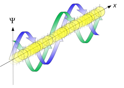
Propagation of free particle waves in 1d - real part of the complex amplitude is blue, imaginary part is green. The probability (shown as the color opacity) of finding the particle at a given point x is spread out like a waveform, there is no definite position of the particle. Image used with permission

Example 5.1

Use the normalization constraint to evaluate \(A_\pm\) in equation \eqref{eq:5.1.18}.

A Property of Linear Differential Equations

• For linear differential equations, linear combinations of solutions are solutions $$ \begin{equation} \psi(x) = C_1\psi_+(x) + C_2 \psi_- (x) \label{eq:5.1.19} \end{equation} $$

Example 5.2

Extract the momentum from the wavefunction for a free electron.

The Energy of the Free Particle

• We can now use the Hamiltonian to determine the energy of the free particle $$ \begin{align} \hat{\mathcal{H}}\psi_\pm(x) &= \frac{-\hbar^2}{2m}\frac{d^2}{dx^2} A_\pm e^{\pm ikx} \\ &= \frac{-\hbar^2}{2m}\left( \pm ik \right)^2 A_\pm e^{\pm ikx} \\ &= \frac{\hbar^2 k^2}{2m} A_\pm e^{\pm ikx} \label{eq:5.1.26} \end{align} $$
• So, we can now see that $$ \begin{equation} E=\frac{\hbar^2 k^2}{2m} \label{eq:5.1.27} \end{equation} $$

Analysis of what we have learned.

• We have not found any restrictions on the momentum or the energy
• These quantities are not quantized for the free particle because there are no boundary conditions
• Any wave with any wavelength fits into an unbounded space
• Quantization results from boundary conditions imposed on the wavefunction, as was the case for the particle-in-a-box
• The probability density of a free particle at a position in space \(x_0\) is $$ \begin{equation} \psi_\pm^*(x_0) \psi_\pm(x_0) = (2L)^{-1} e^{\mp ikx_0} e^{\pm ikx_0} = (2L)^{-1} \label{eq:5.1.28} \end{equation} $$
• This probability is independent of \(x_0\) therefore the electron can be found any place along the x axis with equal probability
• This means that we have no knowledge of the position of the electron, we do, however, know the electron's momentum exactly

The Uncertainty Principle

• In the mid 1920's, Werner Heisenberg showed that if we try to locate an electron within a region \(\Delta x\) by, for instance, scattering light from it, some momentum is transfered to the electron
• However, it is not possible to determine exactly how much momentum is transfered, even in principle
• Heisenberg showed the the relationship between the uncertainty in the position \(\Delta x\) and the uncertainty in momentum \(\Delta p\) must follow $$ \begin{equation} \Delta p \Delta x \ge \frac{\hbar}{2} \label{eq:5.2.1} \end{equation} $$
• As \(\Delta p\) approached zero, \(\Delta x\) approaches \(\infty\)

Linear Combinations of Eigenfunctions

• Is is not necessary that an electron be described by an eigenfunction of the Hamiltonian operator
• Many problems encountered by quantum chemists and computational chemists lead to wavefunctions that are not eigenfunctions of the Hamiltonian operator

Combination Wavefunction

• Consider a free electron in one dimension that is described by $$ \begin{equation} \psi(x)=C_1\psi_1(x)+C_2 \psi_2(x) \label{eq:5.3.1} \end{equation} $$ with $$ \psi_1(x) = \left( \frac{1}{2L}\right)^\frac{1}{2} e^{ik_1 x} $$ $$ \psi_2(x) = \left( \frac{1}{2L}\right)^\frac{1}{2} e^{ik_2 x} $$ where \(k_1\) and \(k_2\) have different magnitudes
• Although such a function is not an eigenfunction of the momentum operator or the Hamiltonian operator, we calculate the average momentum and average energy from the expectation value integrals

Example 5.3

Show that the function \(\psi(x)\) defined by Equation \eqref{eq:5.3.1} is not an eigenfunction of the momentum operator or the Hamiltonian operator for a free electron in one dimension.

Superposition Functions

• Equation \eqref{eq:5.3.1} belong to a class of functions known as superposition functions
• Superposition functions are linear combinations of eigenfunctions
• A linear combination of functions is a sum of functions, each multiplied by a weighting coefficient, which is a constant
• The constants \(C_1\) and \(C_2\) in equation \eqref{eq:5.3.1} give the weight of each component (\(\psi_1\) and \(\psi_2\)) in the total wavefunction

Expectation Value

• We now need to determine the expectation value, ie. average value, of the momentum operator
• First we write the integral for expectation value $$ \begin{align} \expect{p} &= \int_{-L}^{+L} \psi^*(x) \left( -i\hbar \frac{d}{dx} \right) \psi(x) dx \label{eq:5.3.4} \\ &= \frac{-i\hbar}{2L} \int_{-L}^{+L} \left( C_1^* e^{-ik_1 x} + C_2^*e^{-ik_2 x} \right)\frac{d}{dx} \left( C_1 e^{ik_1x}+C_2e^{ik_2x} \right)dx \label{eq:5.3.5} \\ &= \frac{-i\hbar}{2L} \int_{-L}^{+L} \left[ \begin{split} & \left( C_1^* e^{-ik_1 x} + C_2^*e^{-ik_2 x} \right) \\ & \times \left( (ik_1) C_1 e^{ik_1x}+(ik_2)C_2e^{ik_2x} \right) \end{split} \right] dx \label{eq:5.3.6} \end{align} $$

Solving the Integral

• Cross-multiplying the two factors yields four terms $$ \expect{p} = I_1+I_2+I_3+I_4 $$ with $$ \begin{align} I_1 &= \frac{\hbar k_1}{2L} C_1^* C_1 \int_{-L}^{+L} dx = C_1^* C_1 \hbar k_1 \label{eq:5.3.7} \\ I_2 &= \frac{\hbar k_2}{2L} C_2^* C_2 \int_{-L}^{+L} dx = C_2^* C_2 \hbar k_2 \label{eq:5.3.8} \\ I_3 &= \frac{\hbar k_2}{2L} C_1^* C_2 \int_{-L}^{+L} e^{i\left(k_2-k_1\right)x} dx \label{eq:5.3.9} \\ I_4 &= \frac{\hbar k_1}{2L} C_2^* C_1 \int_{-L}^{+L} e^{i\left(k_1-k_2\right)x} dx \label{eq:5.3.10} \end{align} $$

Overlap Integral

• An integral of two different functions (\(\int \psi_1^* \psi_2 dx\)) is called an overlap integral or othogonality integral
• When such an integral equals zero, the functions are said to be orthogonal
• The integrals \(I_3\) and \(I_4\) are zero because the functions \(\psi_1\) and \(\psi_2\) are orthogonal
• We know that they are orthogonal because of the orthogonality theorem
• We can also show it using Euler's formula and following example given in the following example problem

Example 5.4

For the integral part of \(I_3\) obtain $$ \int \cos \left[\left( k_2-k_1\right)x\right]dx + i \int \sin \left[\left(k_2-k_1\right)x\right] dx $$ from Euler's formula $$ e^{\pm ikx} = \cos(kx) \pm i\,\sin(kx) $$