Electronic Spectroscopy of Cyanine Dyes
Shaun Williams, PhD
Cyanine Dyes
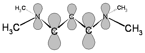
- Cyanine dye molecules are planar cations as shown below
- The number of carbon atoms in the chain an vary
- The R groups represent \(\chem{H}\), \(\chem{CH_3}\), \(\chem{CH_2CH_3}\), or many others including ring structures
- The position (wavelength) and strength (absorption coefficient) of the absorption band depends on the length of the carbon chain but not by the end groups

Absorption Characteristics
- These molecules are called dyes because they have very intense absorption bands in the visible as shown below
- This strong absorption makes solutions of these molecules brightly colored
- A solution of the dye shows the color of the light that is not absorbed
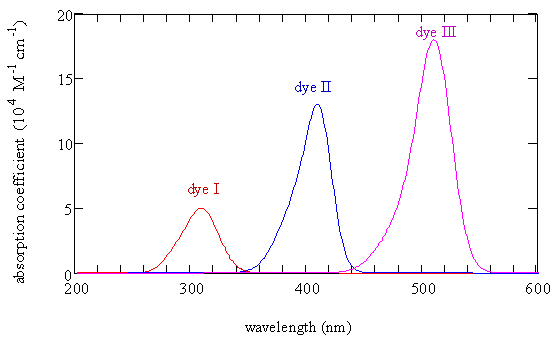 Dye I has 3 carbon atoms and the absorption maximum is at 309 nm, dye II has 5 carbon atoms and the absorption maximum is at 409 nm, and dye III has 7 carbon atoms and the absorption maximum at 512 nm. \(\chem{R=CH_3}\)
Example 4.1
Draw the Lewis electron dot structure of dye I that produced the spectrum shown in the Figure on the previous slide with the maximum absorption at 309 nm. Examine the resonance structures and determine whether all the carbon-carbon bonds are identical or whether some are single bonds and some are double bonds.
Example 4.2
Use the absorption spectra from two slides ago to describe what happens to the maximum absorption coefficient and the wavelength of the peak absorption as the length of a cyanine dye molecule increases.
Cyanine Dye Electrons
- The electrons and bonds in the cyanine dyes can be classified as sigma and pi
- The probability densities for the sigma electrons are large along the lines connecting the nuclei
- The probability densities for the \(\pi\) electrons are large above and below the plane containing the nuclei
- In molecular orbital theory, the \(\pi\) electrons can be described by wavefunctions composed from \(p_z\) atomic orbitals
Example 4.3
Determine the number of pi electrons in each of the three molecules previously described: dye I, dye II, and dye III.
Delocalization
- The pi electrons in these molecules are delocalized over the length of the molecule between the nitrogen atoms
- When UV and visible light is absorbed, the energy is used to cause transitions of the pi electrons from one energy level to another
- The longest wavelength (lowest energy) transition occurs from the highest-energy occupied level to the lowest-energy unoccupied level
- We will use quantum mechanics and a simple model (the particle-in-a-box) to explain why longer molecules absorb at longer wavelengths and have larger absorption coefficients
Potential Energy
- We can visualize the potential energy experienced by the pi electron as varying along the chain as shown below
- This potential effectively traps the electron in the pi region
- At the end of the chain the potential energy rises to a large value
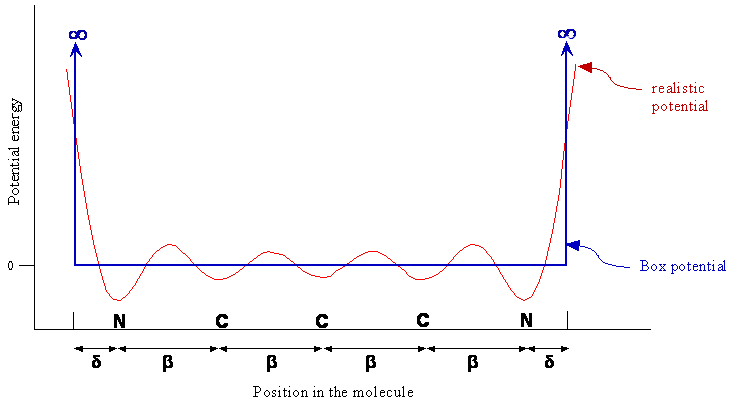
Particle-in-a-Box (PIB) Potential
- The particle-in-a-box model essentially consists of three approximations to the actual potential energy
- The chain of carbon atoms forms a one-dimensional space of some length \(L\) for the pi electrons
- The potential energy is constant along the chain (ie. the oscillations are ignored)
- The potential energy becomes infinite at some point slightly past the nitrogen atoms
- Since only changes in energy are meaningful, and an absolute zero of energy does not exist, the constant potential energy of the electron along the chain between the nitrogen atoms can be defined as zero
The Particle-in-a-Box Model Usages
- The particle-in-a-box model allows us to relate the transition energy obtained from the position of the absorption maximum to the length of the conjugated part of the molecule, \(L\)
- From this length, we can obtain the average bond length \(\beta\) and the distance \(\delta\) the box extends beyond the nitrogen atom
- Some end groups might, due to their polarizability or electronegativity, allow the electrons to penetrate further past the nitrogen atoms
Example 4.4
In the previous potential energy figure, why does a realistic potential energy dip at each atom? Why is the dip larger for nitrogen than for carbon? Why does the potential energy increase sharply at the ends of the molecule?
The Particle-in-a-Box Model
- The particle-in-a-box model is used to approximate the Hamiltonian operator for the \(\pi\) electrons because the full Hamiltonian cannot be solved analytically
- In the full Hamiltonian, the Coulomb potential between interacting electrons cannot be solved
- We want a model for the dye molecules that has a simple potential energy function so we can solve the Schrödinger equation easily
The Particle-in-a-Box Potential
- We are going to assume that the \(\pi\) electron motion is restricted to left and right on the chain in one dimension
- The average potential energy due to interactions is taken to be constant except at the ends of the molecule
- At the ends, the potential rises abruptly to a large value
- We define the constant potential in the box as being zero and the potential outside the box as being infinite.
- So for one electron located in the box, between \(x=0\) and \(x=L\) $$ \begin{equation} \hat{\mathcal{H}}=\frac{-\hbar^2}{2m}\frac{d^2}{dx^2} \label{eq:4.3.2} \end{equation} $$
The Particle-in-a-Box Schrödinger Equation
- Since \(V(x)=0\) inside the box, the Schrödinger equation becomes $$ \begin{equation} \frac{-\hbar^2}{2m}\frac{d^2}{dx^2}\psi(x)=E\psi(x) \label{eq:4.3.3} \end{equation} $$
- We need to solve this differential equation to find the wavefunction and the energy
- In general, differential equations have multiple solutions (solutions that are families of function
- This means that by solving the equation, we will find all the wavefunctions and all the energies for the particle-in-a-box
Example 4.5
Use \( \sin(kx)\), \( \cos(kx)\), and \( e^{ikx} \) for the possible wavefunctions in Equation \eqref{eq:4.3.3} and differentiate twice to demonstrate that each of these functions satisfies the Schrödinger equation for the particle-in-a-box.
First Solutions
- In the previous example we found three equations $$ \frac{\hbar^2 k^2}{2m}\sin(kx)=E\sin(kx) $$ $$ \frac{\hbar^2 k^2}{2m}\cos(kx)=E\cos(kx) $$ $$ \frac{\hbar^2 k^2}{2m}e^{ikx}=Ee^{ikx} $$
- For these equations to be true $$ \begin{equation} E=\frac{\hbar^2k^2}{2m} \label{eq:4.3.7}\end{equation} $$
Boundary Conditions
- Since kinetic energy is \(\frac{p^2}{2m}\) we can conclude that \(\hbar^2k^2=p^2\)
- It is important to know that solutions to differential equations that describe the real world must also satisfy conditions imposed by the physical situation. These conditions are called boundary conditions
- For the particle-in-a-box, the particle is restricted to the region of space between \(x=0\) and \(x=L\)
- Since the potential energy goes to infinity at the boundary, the wavefunctions must be zero at \(x=0\) and \(x=L\)
- This gives us the boundary condition that \(\psi(0)=\psi(L)=0\)
Example 4.6
Which of the functions \(\sin(kx)\), \(\cos(kx)\), or \(e^{ikx}\) is \(0\) when \(x = 0\)?
Satisfying the Boundary Condition
The Particle-in-a-Box Wavefunctions
- The set of wavefunctions that satisfy both boundary conditions is $$ \begin{equation} \psi_n(x) = N\sin \left( \frac{n\pi}{L}x \right)\text{ with } n=1,2,3,\dots \label{eq:4.3.12}\end{equation} $$
- The normalization constant \(N\) is introduced and evaluated to satisfy the normalization requirement $$ \begin{equation} \int_0^L \psi^*(x)\psi(x)dx=1 \label{eq:4.3.13}\end{equation} $$
- Plugging in our wavefunctions $$ \begin{equation} N^2 \int_0^L \sin^2 \left( \frac{n\pi x}{L} \right) dx=1 \label{eq:4.3.14} \end{equation} $$
Normalizing the Wavefunctions
$$ N^2 \int_0^L \sin^2 \left( \frac{n\pi x}{L} \right) dx=1 $$ $$ N=\sqrt{\frac{1}{\int_0^L \sin^2 \frac{n\pi x}{L} dx}} $$ $$ N=\sqrt{\frac{2}{L}} $$ This gives us the wavefunction $$ \begin{equation} \psi_n(x)=\sqrt{\frac{2}{L}}\sin \left( \frac{n\pi}{L} x \right) \label{eq:4.3.17} \end{equation} $$
Example 4.7
Evaluate the integral in Equation \eqref{eq:4.3.14} and show that \(N=\sqrt{\frac{2}{L}}=\left(\frac{2}{L}\right)^{\frac{1}{2}}\)
Summary of the Particle-in-a-Box So Far
- We have found a while set of wavefunctions and corresponding energies for the particle-in-a-box
- The wavefunctions are given by equation \eqref{eq:4.3.17}
- We can find the energy expression by substituting \(k\) from equation \eqref{eq:4.3.9} into equation \eqref{eq:4.3.7} $$ \begin{equation} E_n = \frac{n^2\pi^2\hbar^2}{2mL^2} = n^2 \left( \frac{h^2}{8mL^2} \right) \label{eq:4.3.18}\end{equation} $$
- We see that the energy is quantized in units of \(\frac{h^2}{8mL^2}\)
- Realize that the quantization of the energy has been produced from the boundary conditions.
- The lowest energy state is called the ground state, \(n=1\)
Example 4.8
Substitute the wavefunction, Equation \eqref{eq:4.3.17}, into Equation \eqref{eq:4.3.3} and differentiate twice to obtain the expression for the energy given by Equation \eqref{eq:4.3.18}.
Example 4.9
Here is a neat way to deduce or remember the expression for the particle-in-a-box energies. The momentum of a particle has been shown to be equal to \(\hbar k\). Show that this momentum, with \(k\) constrained to be equal to \(\frac{n\pi}{L}\), combined with the classical expression for the kinetic energy in terms of the momentum \(\left( \frac{p^2}{2m} \right)\) produces Equation \eqref{eq:4.3.18}. Determine the units for \(\frac{h^2}{8mL^2}\) from the units for \(h\), \(m\), and \(L\).
Example 4.10
Why must the wavefunction for the particle-in-a-box be normalized? Show that \( \psi(x)\) in Equation \eqref{eq:4.3.17} is normalized.
Example 4.11
How does the energy of the electron depend on the size of the box and the quantum number \(n\)? What is the significance of these variations with respect to the spectra of cyanine dye molecules with different numbers of carbon atoms and \(\pi\) electrons? Plot \( E(n^2) \), \( E(L^2) \), and \( E(n) \) on the same figure and comment on the shape of each curve.
Spectroscopy of the Particle-in-a-Box Model
- The wavefunction that describe electrons in atoms and molecules are called orbitals
- When we say an electron is in orbital \(n\), we mean that it is described by \(\psi_n\) and has an energy \(E_n\)
- When an atom or molecules absorbs a photon, the atom or molecule goes from one energy level, \(n_i\), to a higher energy level, \(n_f\) - this is called a transition
Orbital Transitions
- The energy of the photon absorbed by the atom or molecule (\(E_{photon}=h\nu\)) matches the difference in energy between the two states involved in the transition \(\Delta E_{states}\) $$ \begin{equation} \Delta E_{states} = E_f-E_i=E_{photon}=h\nu = hc\widetilde{\nu} \label{eq:4.4.1} \end{equation} $$
- For the particle-in-a-box $$ \begin{equation} E_{photon}=\Delta E_{states} = E_f-E_i = \frac{\left( n_f^2 - n_i^2 \right) h^2}{8mL^2} \label{eq:4.4.2} \end{equation} $$ where \(n_i\) is the quantum number of the initial state while \(n_f\) is that of the final state
- If \(E_{photon}\lt 0\) then a photon is emitted and if \(E_{photon} \gt 0\) then a photon is absorbed
Transition Specifics
- Generally the transition energy, \(E_{photon}\), is taken to correspond to the peak in the absorption spectrum
- In a cyanine dye molecule that has 3 carbon atoms in the chain, there are six \(\pi\) electrons
- When light is absorbed, one of these electrons increases its energy by an amount \(h\nu\) and transitions to a higher energy level
- In order to use equation \eqref{eq:4.4.1}, we need to know which energy levels are involved
- We assign electrons to the lowest energy levels to create the ground-state lowest-energy electron configuration
- The Pauli Exclusion Principle says that each spatial wavefunction can describe, at most, two electrons
Empirically Discover the Pauli Exclusion Principle
- When there is an even number of electrons, the lowest-energy transition is the energy different between the highest occupied level (HOMO) and the lowest unoccupied level (LUMO)
- HOMO - highest occupied molecular orbital
- LUMO - lowest unoccupied molecular orbital
- All other transitions have a higher energy
- If all the electrons are in the first energy level, the lowest-energy transition would be \(h\nu=E_2-E_1\)
- With one electron in each of the first six levels, \(h\nu=E_7-E_6\)
- If the electrons are paired, \(h\nu=E_4-E_3\)
Example 4.12
Draw energy level diagrams indicating the HOMO, the LUMO, the electrons and the lowest energy transition for each of the three cases mentioned in the preceding slide.
Example 4.13
For the three ways of assigning the 6 electrons to the energy levels in the previous Example, calculate the peak absorption wavelength \(\lambda\) for a cyanine dye molecule with 3 carbon atoms in the chain using a value for \(L\) of \(0.849\, nm\), which is obtained by estimating bond lengths. Which wavelength agrees most closely with the experimental value of \(309\, nm\) for this molecule?
Final Notes about Transitions
- In the previous examples we have "discovered" the Pauli Exclusion Principle
- electrons should be paired in the same energy level whenever possible
- In molecules with an odd number of electrons
- it is possible to have transitions between the doubly occupied molecular orbitals and a singly occupied molecular orbital
- it is possible to have a transition from the singly occupied orbital to an unoccupied orbital
The Transition Dipole Moment and Spectroscopic Selection Rules
- We can now deal with what energy level transitions are possible
- Clearly the transition cannot violate the Pauli Exclusion Principle
- There are additional restrictions that result from the nature of the interaction between electromagnetic radiation and matter - these are selection rules
Beginning to Obtain the Selection Rules
- We first consider light as consisting of perpendicular oscillating electric and magnetic fields
- The magnetic field interacts with magnetic moments and causes transitions seen in electron spin resonance and nuclear magnetic resonance spectroscopies
- The oscillating electric field interacts with electrical charges and causes transitions seen in the UV-visible, atomic absorption, and fluorescence spectroscopies
The Interaction
- The energy of interaction, \(E\), between a system of charged particles and an electric field \(\varepsilon\) is given by the scalar product of the electric field and the dipole moment, \(\mu\), for the system (both are vectors) $$ \begin{equation} E=-\mu\cdot \varepsilon \label{eq:4.5.1} \end{equation} $$
- The dipole moment is defined as the summation of the product of the charge \(q_j\) times the position vector \(r_j\) for all charged particles \(j\) $$ \begin{equation} \mu = \sum_j q_jr_j \label{eq:4.5.2} \end{equation} $$
Example 4.14
Calculate the dipole moment of \(\chem{HCl}\) from the following information. The position vectors below use Cartesian coordinates \((x, y, z)\), and the units are \(pm\). What fraction of an electronic charge has been transferred from the chlorine atom to the hydrogen atom in this molecule? \( r_H=(124.0,0,0)\), \(r_{Cl}=(−3.5,0,0)\), \(q_H=2.70\times 10^{−20}C\), \(q_{Cl}=−2.70\times 10^{−20}C\).
Interaction Energy
- We need to calculate an expectation value for this interaction energy $$ \begin{equation} \expect{E} = \int \psi_n^* \left( -\hat{\mu} \cdot \hat{\varepsilon} \right)\psi_n d\tau \label{eq:4.5.3} \end{equation} $$
- The operators \(\hat{\mu}\) and \(\hat{\varepsilon}\) are vectors and are the same as the classical quantities \(\mu\) and \(\varepsilon\)
- Usually the wavelength of light used in electronic spectroscopy is very long compared to the length of a molecule thus the electric field is essentially constant over the length of the molecule so that \(\varepsilon\) can come out of the integral
- Effectively, what remains is $$ \begin{equation} \expect{E} = -\expect{\mu} \cdot \varepsilon \text{ where } \expect{\mu} = \int \psi_n^* \hat{\mu} \psi_n d\tau \label{eq:4.5.4} \end{equation} $$
Transition Dipole Moment
- To obtain the strength of the interaction, the transition dipole moment is used rather than the dipole moment
- The transition dipole moment integral is very similar to the dipole moment given in equation \eqref{eq:4.5.4} except the two wavefunctions are different
- For a transition where the state changes from \(\psi_i\) to \(\psi_f\), the transition dipole moment integral is $$ \begin{equation} \expect{\mu}_T = \int \psi_f^* \hat{\mu} \psi_i d\tau = \mu_T \label{eq:4.5.6} \end{equation} $$
- The probability for a transition is measured by the absorption coefficient is proportional to the absolute square \(\mu_T^*\mu_T\)
Analyzing the Transition Dipole Moment
- If \(\mu_T=0\) then the interaction energy in zero and no transition occurs - these transitions are said to be forbidden
- If \(\mu_T\) is large then the probability for a transition and the absorption coefficient are large
- We need to find a way of determining if \(\mu_T\ne 0\) or \(\mu_T=0\) without having to evaluate the integrals
- To do this we can use properties such a wavefunction symmetry and angular momentum
- This evaluation leads to selection rules with summarize the conditions where \(\mu_T\ne 0\) - they do not say how probable or intense the transition is
- For our one-dimensional particle in a box we need to evaluate $$ \begin{equation} \mu_T = -e\int_0^L \psi_f^*(x) x \psi_i(x) dx \label{eq:4.5.7} \end{equation} $$
Selection Rules for the Particle-in-a-Box
- Let's plug our particle-in-a-box wavefunction \eqref{eq:4.3.17} into our integral, \eqref{eq:4.5.7} $$ \begin{align} \mu_T &= -e \int_0^L \sqrt{\frac{2}{L}} \sin \left( \frac{n_f \pi x}{L} \right) x \sqrt{\frac{2}{L}} \sin \left( \frac{n_i \pi x}{L} \right) dx \label{eq:4.6.1} \\ &= \frac{-2e}{L} \int_0^L x \sin \left( \frac{n_f \pi x}{L} \right) \sin \left( \frac{n_i \pi x}{L} \right) dx \label{eq:4.6.2} \end{align} $$
Simplifying Our Integral
- We can simplify our integral by using the relation: $$ \sin \psi \sin \theta = \frac{1}{2}\left[ \cos (\psi-\theta) - \cos (\psi+\theta) \right] $$ as well as by defining $$ \Delta n = n_f-n_i \text{ and } n_T=n_f+n_i $$
- This results in $$ \begin{align} \mu_T &= \frac{-e}{L} \int_0^L x \left[ \cos \left( \frac{\Delta n \pi x}{L} \right) - \cos \left( \frac{n_T \pi x}{L} \right) \right] dx \label{eq:4.6.4} \\ &= \frac{-e}{L} \left[ \int_0^L x \cos \left( \frac{\Delta n \pi x}{L} \right) dx - \int_0^L x \cos \left( \frac{n_T \pi x}{L} \right) dx \right] \label{eq:4.6.5} \end{align} $$
Integral Evaluation
- We can evaluate that integral using integral tables (which can be found by doing an internet search to "integral tables") $$ \int_0^L x\cos(ax)dx = \left[ \frac{1}{a^2}\cos(ax)+\frac{x}{a}\sin(ax) \right]_0^L $$ where \(a\) is any nonzero constant
- Plugging this in we get $$ \begin{equation} \mu_T=\frac{-e}{L}\left( \frac{L}{\pi} \right)^2 \left[ \begin{split} & \frac{1}{\Delta n^2} (\cos (\Delta n \pi)-1) - \frac{1}{n_T^2}(\cos(n_T \pi)-1) \\ & + \frac{1}{\Delta n}\sin (\Delta n \pi)-\frac{1}{n_T}\sin(n_T \pi) \end{split} \right] \label{eq:4.6.7} \end{equation} $$
Example 4.15
Show that if \(\Delta n\) is an even integer, then \(n_T\) must be an even integer and \(\mu_T=0\).
Example 4.16
Show that if \(n_i\) and \(n_f\) are both even or both odd integers then \(\Delta n\) is an even integer and \(\mu_T=0\).
Example 4.17
Show that if \(\Delta n\) is an odd integer, then \(n_T\) must be an odd integer and \(\mu_T\) is given by equation \eqref{eq:4.6.8}. $$ \begin{equation} \mu_T = \frac{-2eL}{\pi^2} \left( \frac{1}{n_T^2}-\frac{1}{\Delta n^2} \right) = \frac{8eL}{\pi^2}\left( \frac{n_fn_i}{\left( n_f^2-n_i^2\right)^2} \right) \label{eq:4.6.8} \end{equation} $$
Example 4.18
What is the value of the transition moment integral (equation \eqref{eq:4.6.7}) for the transitions \(1\rightarrow 3\) and \(2\rightarrow 4\)?
Example 4.19
What is the value of the transition moment integral, equation \eqref{eq:4.6.7}, for transitions \(1\rightarrow 2\) and \(2\rightarrow 3\)?
The Particle-in-a-Box Selection Rule
- From the preceding examples and examples, we can formulate the selection rules for the particle-in-a-box model
- Transitions are forbidden if \(\Delta n = n_f-n_i\) is an even integer
- Transitions are allowed if \(\Delta n=n_f-n_i\) is an odd integer
Example 4.20
The lowest energy transition is from the HOMO to the LUMO, which were defined previously. Compute the value of the transition moment integral for the HOMO to LUMO transition \(E_3\rightarrow E_4\) for a cyanine dye with 3 carbon atoms in the conjugated chain. What is the next lowest energy transition for a particle-in-a-box? Compute the value of the transition moment integral for the next lowest energy transition that is allowed for this dye. What are the quantum numbers for the energy levels associated with this transition? How does the probability of this transition compare in magnitude with that for \( 3\rightarrow 4\)?
Using Symmetry to Identify Integrals that are Zero
- It generally required a lot of time and effort to evaluate integral
- This can be saved if we can quickly identify by inspection when integrals are zero
- We are going to examine the properties of wavefunctions for a particle-in-a-box to determine when \(\mu_T\) is zero
- These considerations are general and can be applied to any integrals
Particle-in-a-Box Coordinate System
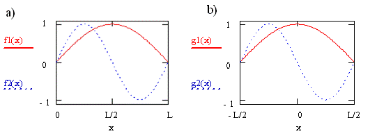
- The wavefunctions for \(n=1\) and \(n=2\) are shown in the left of the figure above
- Notice that when we shift the axis system so that the wavefunction is centered at 0, the wavefunctions do not change (right side in the figure)
- After shifting the coordinate system the barriers are at \(\pm\frac{L}{2}\)
- While the probability does not change, the functions do (they change from \(\cos\) to \(-\sin\))
Why did we shift the coordinates?
- We moved the origin of the coordinate system to the center of the box to take advantage of the symmetry properties of the functions
- By symmetry we mean the correspondence in form other either side of a dividing point, line, or plane.
- Analysis of symmetry is straightforward is the origin of the coordinates coincides with the dividing point, line, or plane
- Since the right and left halves of the box or molecule are the same, the square of the wavefunction for \(x \gt 0\) must be the same as the square of the wavefunction for \(x\lt 0\)
- In English this means that there is no reason that the particle described by the wavefunction would prefer one side of the box to the other
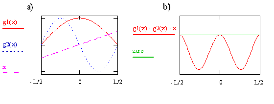
The First Symmetry Analysis of \(\mu_T\)
- The transition moment integral for the particle-in-a-box involves the product of three function \(\psi_f\), \(\psi_i\), and \(x\)
- For \(n_i=1\) and \(n_f=2\), the plots are in the below figure on the left
- The product of the three functions is given on the right
- The value of the integral is the sum of the area between the product and the zero baseline
- Clearly, in this case, that sum is less than zero (and not equal to zero) - the transition is allowed
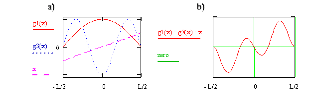
Another Symmetry Analysis of \(\mu_T\)
- Now we consider \(n_i=1\) and \(n_f=3\), the plots are in the below figure on the left
- The product of the three functions is given on the right
- As can be seen, the product (integrand) is negative for \(x\lt 0\) and positive for \(x \gt 0\)
- The overall effect is that the cancel out - the net negative and the net positive are equal and opposite so their sum is zero
- This means that this transition is forbidden
New Spectroscopy Terms
- In spectroscopy we have some special terms used to describe the symmetry properties of wavefunctions
- The terms "symmetric", "gerade", and "even" describe functions like \(f(x)=x^2\) and \(\psi_1(x)\) - that is, they are functions in which \(f(x)=f(-x)\)
- The terms "antisymmetric", "ungerade", and "odd" describe functions like \(f(x)=x\) and \( \psi_2(x)\) - that is, they are functions in which \(f(x)=-f(-x)\)
- Gerade and ungerade are German words meaning even and odd and are abbreviated \(g\) and \(u\)
- It is important to note that antisymmetric does not mean non-symmetric
- In an integrand is \(u\), then the integral is zero - the integrand is \(u\) is the product of the functions comprising it is \(u\)
- The following rules make it possible to quickly identity whether a product of two functions is \(u\) $$ g\cdot g=g,\;u\cdot u=g,\; g\cdot u=u $$
Example 4.21
Use symmetry arguments to determine which of the following transitions between quantum states are allowed for the particle-in-a-box: \(n = 2\) to \(3\) or \(n = 2\) to \(4\).
Other Properties of the Particle-in-a-Box
- We are now going to approach answering some interesting questions
- What is the lowest energy for an electron?
- The lowest energy level is \(E_1\) and it is important to recognize that this lowest energy is not zero
- This finite (meaning neither zero nor infinite) energy is called the zero-point energy and the motion associated with this energy is called the zero-point motion
- Zero-point energy and the associated motion are manifestations of the wave properties and the Heisenberg Uncertainty Principle, and are general properties of bound quantum mechanical systems
The Heisenberg Uncertainty Principle
- The position and momentum of the particle cannot be determined exactly
- According to the Heisenberg Uncertainty Principle, the product of the uncertainties in position and momentum must be greater than or equal to \(\frac{\hbar}{2}\)
- If the energy were zero, then the momentum would be exactly zero which would violate the Heisenberg Uncertainty Principle unless the uncertainty in position were infinite
- Infinite uncertainty in position means that the system is not localized in space at all which cannot be true for a bound system
Example 4.22
Use the general form of the particle-in-a-box wavefunction \(\sin(kx)\) for any \(n\) to find the mathematical expression for the position expectation value \(\expect{x}\) for a box of length \(L\). How does \(\expect{x}\) depend on \(n\)? Evaluate the integral.
Example 4.23
Show that the particle-in-a-box wavefunctions are not eignfunctions of the momentum operator.
Example 4.24
Even though the wavefunctions are not momentum eigenfunctions, we can calculate the expectation value for the momentum. Show that the expectation or average value for the momentum of an electron in the box is zero in every state.
The Momentum
- Even though it may seem that the electron does not have any momentum, that cannot be correct since we know the energy is never zero
- In fact, the energy that we obtained for the particle-in-a-box is entirely kinetic energy because we set the potential energy to zero
- Since kinetic energy is momentum squared divided by twice the mass, we can determine how the average momentum is zero so that the kinetic energy is finite
- It must be equally likely for a particle-in-a-box to have a momentum of \(-p\) are \(+p\)
- While the average of \(-p\) and \(+p\) is zero, the sum of the squares is nonzero
- Does the fact that the average momentum of an electron is zero and the average position is \(\frac{L}{2}\) violate the Heisenberg Uncertainty Principle? No, because the Heisenberg Uncertainty Principle pertains to the uncertainty in the momentum and in the position, not to the average values
Looking at the Uncertainties
- Let's look at the root mean square deviation from the averages
- The standard deviation in the position of the particle-in-a-box is given by $$ \begin{equation} \sigma_x = \frac{L}{2\pi n} \sqrt{\frac{\pi^2}{3}n^2-2} \label{eq:4.8.6} \end{equation} $$
- The standard deviation in the momentum is $$ \begin{equation} \sigma_p = \frac{n\pi \hbar}{L} \label{eq:4.8.7} \end{equation} $$
Example 4.25
Evaluate the product \(\sigma_x \cdot \sigma_p\) for \(n = 1\) and for general \(n\). Is the product greater than \(\frac{\hbar}{2}\) for all values of \(n\) and \(L\) as required by the Heisenberg Uncertainty Principle?
Orthogonality
- Are the eigenfunctions of the particle-in-a-box Hamiltonian orthogonal?
- Two functions, \(\psi_A\) and \(\psi_B\), are orthogonal if $$ \int_{allspace} \psi_A^* \psi_B d\tau = 0 $$
- In general, eigenfunctions of a quantum mechanical operator with different eigenvalues are orthogonal
Example 4.26
Evaluate the integral \(\int \psi_1^* \psi_3 dx\) and as many other pairs of particle-in-a-box eigenfunctions as you wish (use symmetry arguments whenever possible) and explain what the results say about orthogonality of the functions.
Example 4.27
What happens to the energy level spacing for a particle-in-a-box when \( mL^2\) becomes much larger than \(h^2\)? What does this result imply about the relevance of quantization of energy to baseballs in a box between the pitching mound and home plate? What implications does quantum mechanics have for the game of baseball in a world where \(h\) is so large that baseballs exhibit quantum effects?
Determining the Relative Energies of Wavefunctions by Examination
- The first derivative is the rate of change of the functions and the second derivative is the rate of change in the rate of change (also known as the curvature)
- A function with a large second derivative is changing very rapidly
- Since the second derivative is in the Hamiltonian, a wavefunction that has a sharper curvature than another should correspond to a higher energy state
- A wavefunction with more nodes than another over the same region of space must have sharper curvatures and larger second derivatives and therefore should have a higher energy
Properties of Quantum Mechanical Systems
- As we have analyzed the particle-in-a-box model, we have bound some important properties of quantum mechanical systems
- We saw that the eigenfunctions of the Hamiltonian operator are orthogonal
- We saw that the position and momentum of the particle could not be determined exactly
- We are now going to prove some fundamental theorems
Hermitian Theorem
- Since the eigenvalues of a quantum mechanical operator correspond to measurable quantities, the eigenvalues must be real, and consequently a quantum mechanical operator must be Hermitian
- We start with the premise that \(\psi\) and \(\phi\) are functions, \(\int d\tau\) represents integration over all coordinates, and the operator \(\hat{A}\) is Hermitian by definition if $$ \int \psi^* \hat{A} \psi d\tau = \int \left( \hat{A}^* \psi^* \right) \psi d\tau $$
- Let's prove that quantum mechanical operator \(\hat{A}\) is Hermitian
Hermitian Proof - 1
- Consider the eigenvalue equation and its complex conjugate $$ \hat{A}\psi = a\psi $$ $$ \hat{A}^*\psi^* = a^*\psi^* = a\psi^* $$ Note that \(a^*=a\) because the eigenvalue is real
- Multiply these two equations from the left by \(\psi^*\) and \(\psi\) respectively and integral over all the coordinates (note that \(\psi\) is normalized $$ \int \psi^* \hat A \psi d\tau = a\int \psi^* \psi d\tau =a $$ $$ \int \psi \hat{A}^*\psi^* d\tau = a\int \psi \psi^* d\tau = a $$
Hermitian Proof - 2
- Since both integrals equal \(a\), they must be equivalent $$ \int \psi^* \hat{A}\psi d\tau = \int \psi \hat{A}^* \psi^* d\tau $$
- The operator acting on a function produces a new function and since functions commute we can rewrite this as $$ \int \psi^* \hat{A} \psi d\tau = \int \left(\hat{A}^*\psi^* \right)\psi d\tau $$
- This equality means that \(\hat{A}\) is Hermitian
Othogonality Theorem
- Eigenfunctions of a Hermitian operator are orthogonal if they have different eigenvalues
- Because of this theorem, we can identify orthogonal functions easily without having to integrate or conduct an analysis based on symmetry or other considerations
Orthogonality Theorem Proof - 1
- Let \(\psi\) and \(\psi^*\) are two eigenfunctions of the operator \(\hat{A}\) with real eigenvalues \(a_1\) and \(a_2\), respectively
- Since the eigenvalues are real, \(a_1^*=a_1\) and \(a_2^*=a_2\) $$ \hat{A}\psi = a_1\psi $$ $$ \hat{A}^*\psi^* = a_2\psi^* $$
- Multiplying in on the left and integrating we get $$ \int \psi^* \hat{A}\psi d\tau = a_1 \int \psi^* \psi d\tau $$ $$ \int \psi \hat{A}^*\psi^* d\tau = a_2 \int \psi \psi^* d\tau $$
Orthogonality Theorem Proof - 2
- Now we subtract the left sides and the right sides $$ \int \psi^* \hat{A} \psi d\tau - \int \psi \hat{A}^*\psi^* d\tau = \left( a_1 - a_2 \right)\int \psi^* \psi d\tau $$
- Because \(\hat{A}\) is Hermitian, the left-hand side is zero $$ 0 = \left( a_1-a_2 \right) \int \psi^*\psi d\tau $$
- For this to be true, either \(a_1-a_2=0\) or \(\int \psi^* \psi d\tau=0\)
- If \(a_1\) and \(a_2\) are not equal, then the integral must be zero
- This result proves that nondegenerate eigenfunctions of the same operator are orthogonal
Schmidt Orthogonalization Theorem
- If the eigenvalues of two eigenfunctions are the same, then the functions are said to be degenerate
- Also, linear combinations of the degenerate functions can be formed that will be orthogonal to each other
- Since the two eignefunctions have the same eigenvalues, the linear combination also will be an eigenfunction with the same eigenvalue
- Degenerate eigenfunctions are not automatically orthogonal but can be made so mathematically
Schmidt Orthogonalization Theorem Proof
- If \(\psi\) and \(\phi\) are degenerate but not orthogonal, define \(\Phi=\phi-S\psi\) where \(S\) is the overlap integral \(\int \psi^*\phi d\tau\), then \(\psi\) and \(\Phi\) will be orthogonal $$ \int \psi^* \ \Phi d\tau = \int \psi^* \left(\phi-S\psi\right) d\tau = \int \psi^* \phi d\tau - S \int \psi^* \psi d\tau $$ $$ = S-S=0 $$
Commuting Operator Theorem
- If two operators commute, then they can have the same set of eigenfunctions
- By definition, two operators \(\hat{A}\) and \(\hat{B}\) commute if the effect of applying \(\hat{A}\) and \(\hat{B}\) is the same as applying \(\hat{B}\) then \(\hat{A}\)
- This means that we have to check that \(\hat{A}\hat{B}=\hat{B}\hat{A}\)
- This theorem is very important because if two operators commute and consequently have the same set of eigenfunctions, the the corresponding physical quantities can be evaluated or measured exactly simultaneously with no limit on uncertainty
Commuting Operator Theorem Proof - 1
- If \(\hat{A}\) and \(\hat{B}\) commute and \(\psi\) is an eigenfunction of \(\hat{B}\) with eigenvalue \(b\), then $$ \hat{B}\hat{A}\psi = \hat{A}\hat{B}\psi = \hat{A}b\psi = b\hat{A}\psi $$
- This equation says that at most, \(\hat{A}\) operating on \(\psi\) can produce a constant times \(\psi\) $$ \hat{A}\psi = a\psi $$ $$ \hat{B}(\hat{A}\psi) = \hat{B}(a\psi)=a\hat{B}\psi = ab\psi = b(a\psi) $$
General Heisenberg Uncertainty Principle
- Though it will not be proven here, there is a general statement of the uncertainty principle in terms of the commutation property of operators
- If two operators \(\hat{A}\) and \(\hat{B}\) do not commute, then the uncertainties (standard deviations \(\sigma\)) in the physical quantities associated with these operators must satisfy $$ \begin{equation} \sigma_A \sigma_B \ge \frac{1}{2} \left| \int \psi^* \left[ \hat{A}\hat{B} - \hat{B}\hat{A} \right] \psi d\tau \right| \label{eq:4.9.21} \end{equation} $$
- If \(\hat{A}\) and \(\hat{B}\) commute, then the right-hand side of the above equation is zero so \(\sigma_A\) and/or \(\sigma_B\) are zero
- Thus there are no restrictions on the uncertainties in the measurements of the eignevalues \(a\) and \(b\)
Example 4.28
Show that the commutator for position and momentum in one dimension equals \( i \hbar\) and that the right-hand-side of Equation \eqref{eq:4.9.21} therefore equals \( \frac{\hbar}{2} \) giving \( \sigma_x \sigma_{p_x} \ge \frac{\hbar}{2}\)
Overview of Key Concepts for the Particle in a Box
| Quantity | Value |
|---|---|
| Potential Energy | $$ V = \left\{ \begin{split} & 0 \text{ for }0\lt x \lt L \\ & \infty \text{ otherwise} \end{split} \right. $$ |
| Hamiltonian | \( \hat{\mathcal{H}}=-\frac{\hbar^2}{2m}\frac{d^2}{dx^2} \) |
| Wavefuntions | \( \left( \frac{2}{L} \right)^\frac{1}{2} \sin \left( \frac{n\pi}{L} x \right) \) |
| Quantum Numbers | \( n=1,2,3,\dots \) |
| Energies | \( E=n^2 \left( \frac{h^2}{8mL^2} \right) \) |
| Spectroscopic Selection Rules | \( \Delta n = \text{odd integer} \) |
| Angular Momentum Properties | none |
/