Metals and Alloys - Structure, Bonding, Electronic, and Magnetic Properties
Shaun Williams, PhD
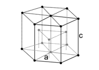
Unit Cells and Crystal Structures
- Crystals can be thought of as repeating patterns in three dimensions.
- The fundamental repeating unit of the crystal is called the unit cell.
We will see that pure metals typically have very simple crystal structures with cubic or hexagonal unit cells.
- However the crystal structures of alloys can be quite complicated.
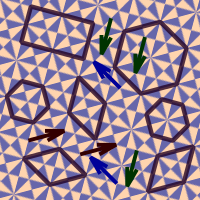
Repetitive Patterns by Tile Groups in a Tiling
Delocalized Electrons
- When considering the crystal structures of metals and alloys, it is not sufficient to think of each atom and its neighboring ligands as an isolated system.
- Instead, think of the entire metallic crystal as a network of atoms connected by a sea of shared valence electrons.
- The electrons are delocalized because there are not enough of them to fill each "bond" between atoms with an electron pair.
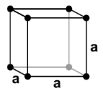
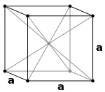
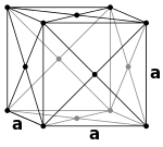
The Unit Cell
- Metal atoms can be approximated as spheres, and therefore are not 100 % efficient in packing
- Different unit cells have different packing efficiencies.
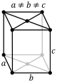
- The number of atoms that is included in the unit cell only includes the fractions of atoms inside of the box. Atoms on the corners of the unit cell count as \(\frac{1}{8}\) of an atom, atoms on a face count as \(\frac{1}{2}\), an atom in the center counts as a full atom.
| Simple Cubic |
Body Centered Cubic |
Face Centered Cubic |
Hexagonal Close Packed |
 |
 |
 |
 |
| 1 atom/cell |
2 atoms/cell |
4 atoms/cell |
2 atoms/cell |
Simple Cubic
- \( 8 \text{ corner atoms}\times \frac{1}{8} = 1\text{ atom/cell}\)
- The packing in this structure is not efficient (52%) and so this structure type is very rare for metals.
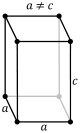
Body Centered Cubic (bcc)
- \(8\text{ corner atoms}\times \frac{1}{8} + 1\text{ center atom}\times 1= 2\text{ atoms/cell}\).
- The packing is more efficient (68%) and the structure is a common one for alkali metals and early transition metals.
- Alloys such as brass (CuZn) also adopt these structures.
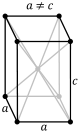
Face Centered Cubic (fcc)
- Also called cubic close packed (ccp)
- \(8\text{ corner atoms}\times \frac{1}{8}+ 6\text{ face atoms}\times \frac{1}{2}= 4\text{ atoms/cell}\)
- This structure, along with its hexagonal relative (hcp), has the most efficient packing (74%).
- Many metals adopt either the fcc or hcp structure.
Hexagonal Close Packed (hcp)
- Like the fcc structure, the packing density of hcp is 74%.
Example 7.1: Packing Efficiency of a Simple Cubic Unit Cell
Calculate the packing efficiency of a simple cubic unit cell.
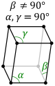
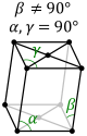
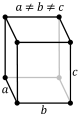
Bravais Lattices
- Crystal lattices can be classified by their translational and rotational symmetry.
- In three-dimensional crytals, these symmetry operations yield 14 distinct lattice types which are called Bravais lattices.
- The fourteen Bravais lattices fall into seven crystal systems that are defined by their rotational symmetry.
- In the lowest symmetry system (triclinic), there is no rotational symmetry - the unit cell edges have equal lengths, and none of the angles are \(90^\circ\).
Bravais Lattice Translational Symmetry
- Primitive (P): lattice points on the cell corners only.
- Body (I): one additional lattice point at the center of the cell.
- Face (F): one additional lattice point at the center of each of the faces of the cell.
- Base (A, B or C): one additional lattice point at the center of each of one pair of the cell faces.
- When the fourteen Bravais lattices are combined with the 32 crystallographic point groups, we obtain the 230 space groups.
- These space groups describe all the combinations of symmetry operations that can exist in unit cells in three dimensions.
- For two-dimensional lattices there are only 17 possible plane groups, which are also known as wallpaper groups.
Lattice Properties
| The 7 Lattice Systems |
The 14 Bravais Lattices |
| Triclinic |
P |
|
|
|
 |
|
|
|
| Monoclinic |
P |
C |
|
|
 |
 |
|
|
| Orthorhombic |
P |
C |
I |
F |
 |
 |
 |
 |
Lattice Properties Continued
| The 7 Lattice Systems |
The 14 Bravais Lattices |
| Tetragonal |
P |
I |
|
|
 |
 |
|
|
| Rhombohedral |
P |
|
|
|
 |
|
|
|
| Hexagonal |
P |
|
|
|
 |
|
|
|
Lattice Properties Concluded
| The 7 Lattice Systems |
The 14 Bravais Lattices |
| Cubic |
P (pcc) |
I (bcc) |
F (fcc) |
|
 |
 |
 |
|
Crystal Structures of Metals
- All metallic elements (except Cs, Ga, and Hg) are crystalline solids at room temperature.
- Like ionic solids, metals and alloys have a very strong tendency to crystallize
- Metals crystallize readily and it is difficult to form a glassy metal even with very rapid cooling.
- Molten metals have low viscosity, and the identical (essentially spherical) atoms can pack into a crystal very easily.
- Glassy metals can be made, however, by rapidly cooling alloys, particularly if the constituent atoms have different sizes.
Crystal Structures
- Most metals and alloys crystallize in one of three very common structures: body-centered cubic (bcc), hexagonal close packed (hcp), or cubic close packed (ccp, also called face centered cubic, fcc).
- In all three structures the coordination number of the metal atoms (i.e., the number of equidistant nearest neighbors) is rather high: 8 for bcc, and 12 for hcp and ccp.
- We can contrast this with the low coordination numbers (i.e., low valences - like 2 for O, 3 for N, or 4 for C) found in nonmetals.
- In the bcc structure, the nearest neighbors are at the corners of a cube surrounding the metal atom in the center.
Atom Stacking
- In the hcp and ccp structures, the atoms pack like stacked cannonballs or billiard balls, in layers with a six-coordinate arrangement.
- Each atom also has six more nearest neighbors from layers above and below.
- The stacking sequence is
- ABCABC in the ccp lattice
- ABAB in in hcp
- In both cases, it can be shown that the spheres fill 74% of the volume of the lattice.
- This is the highest volume fraction that can be filled with a lattice of equal spheres.
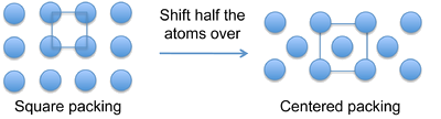
Hexagonal Close Packing (hcp)
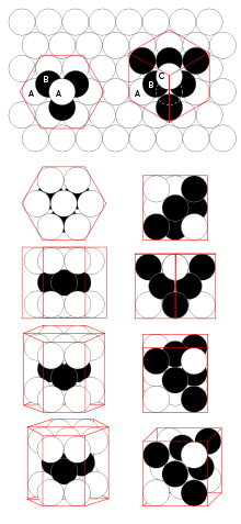
Shifting A Row
Periodic Trends in Structure and Metallic Behavior
- Remember where we find the metallic elements in the periodic table - everywhere except the upper right corner.
- This means that as we go down a group in the p-block (e.g., Group 14, the carbon group, or Group 15, the nitrogen group), the properties of the elements gradually change from nonmetals to metalloids to metals.
- The carbon group nicely illustrates the transition.
- Starting at the top, the element carbon has two stable allotropes. In each one, the valence of carbon atoms is exactly satisfied by making four electron pair bonds to neighboring atoms.
- In graphite, each carbon has three nearest neighbors, and so there are two single bonds and one double bond.
- In diamond, there are four nearest neighbors situated at the vertices of a tetrahedron, and so there is a single bond to each one.
The Elements Under Carbon
- The two elements right under carbon (silicon and germanium) in the periodic table also have the diamond structure
- While diamond is a good insulator, both silicon and germanium are semiconductors (i.e., metalloids).
- Mechanically, they are hard like diamond.
- The next element under germanium is tin (Sn).
- Tin has two allotropes, one with the diamond structure, and one with a slightly distorted bcc structure.
- The bcc structure has metallic properties (metallic luster, malleability), and conductivity about \(10^9\) times higher than Si.
- Finally, lead (Pb), the element under Sn, has the ccp structure, and also is metallic.
Structures and Conductive Properties of Group 14
| Element |
Structure |
Coord. No. |
Conductivity |
| C |
graphite, diamond |
3, 4 |
semimetal, insulator |
| Si |
diamond |
4 |
semiconductor |
| Ge |
diamond |
4 |
semiconductor |
| Sn |
diamond, distorted bcc |
4, 8 |
semiconductor, metal |
| Pb |
ccp |
12 |
metal |
The Electrons in Group 14
- The elements C, Si, and Ge obey the octet rule, and we can easily identify the electron pair bonds in their structures.
- Sn and Pb, on the other hand, adopt structures with high coordination numbers.
- They do not have enough valence electrons to make electron pair bonds to each neighbor.
- In this case is that the valence electrons become "smeared out" or delocalized over all the atoms in the crystal.
- In a metal, an atom's nearest neighbors surround it in every direction, rather than in a few particular directions.
- Nonmetals (insulators and semiconductors), on the other hand, have directional bonding.
- Because the bonding in metals is non-directional and coordination numbers are high, it is relatively easy to deform the coordination sphere (i.e., break or stretch bonds) than it is in the case of a nonmetal.
Bonding in Metals
- The electron pair description of chemical bonds, which was the basis of the octet rule for p-block compounds, breaks down for metals.
- This is illustrated well by Na metal
- Na has too few valence electrons to make electron pair bonds between each pair of atoms.
- We could think of the Na unit cell as having eight no-bond resonance structures in which only one Na-Na bond per cell contains a pair of electrons.
Band Theory
- A more realistic way to describe the bonding in metals is through band theory.
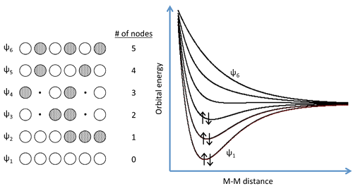
- The evolution of energy bands in solids from simple MO theory is illustrated on the next slide.
- In general, n atomic orbitals (in this case the six Na 3s orbitals) will generate n molecular orbitals with n-1 possible nodes.
- Previously we showed that the energy versus internuclear distance graph for a two hydrogen atom system has a low energy level and a high energy level corresponding to the bonding and antibonding molecular orbitals, respectively.
- These two energy levels were well separated from each other
- If more atoms are introduced to the system, there will be a number of additional levels between the lowest and highest energy levels.
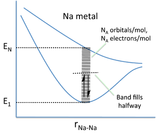
The MO Structure of \(Na_6\)
Expanding Our System to Macroscale
- In band theory, the atom chain is extrapolated to a very large number - on the order of \(10^{22}\) atoms in a crystal - so that the different combinations of bonding and anti-bonding orbitals create "bands" of possible energy states for the metal.
- The number of atoms is so large that the energies can be thought of as a continuum rather than a series of distinct levels.
- A metal will only partially fill this band, as there are fewer valence electrons than there are energy states to fill.
- In the case of Na metal, this results in a half-filled 3s band.
The Band in Na
Nearly Free Electron Model
- In metals, the valence electrons are delocalized over many atoms.
- The total energy of each electron is given by the sum of its kinetic and potential energy:
\[ E=KE+PE \]
\[ E \approx \frac{p^2}{2m} + V \]
where \(p\) is the momentum of the electron (a vector quantity), \(m\) is its mass, and \(V\) is an average potential that the electron feels from the positive cores of the atoms.
- This potential holds the valence electrons in the crystal but, in the free electron model, is essentially uniform across the crystal.
Electron Wavelength and Wavenumber
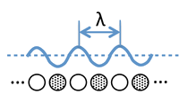
- For a hypothetical infinite chain of Na atoms, the molecular orbitals at the bottom of the 3s band are fully bonding and the wavelength of electrons (2x the distance between nodes) in these orbitals is very long.
- At the top of the band, the highest orbital is fully antibonding and the wavelength is 2 times the distance between atoms (2a), since there is one node per atom.
- Remember that the wavelength of an electron (\(\lambda\)) is inversely proportional to its momentum \(p\), according to the de Broglie relation \(\lambda=\frac{h}{p}\).
- For a (nearly) free electron, the kinetic energy is given by \( KE=\frac{p^2}{2m}=\frac{h^2}{2m\lambda^2} \)
- It is convenient to define the wavenumber of the electron as \(k\), which has units of inverse length and is inversely proportional to \(\lambda\).
- \(k\) is also directly proportional to the momentum \(p\), \( k=2\pi \lambda = 2\pi p h \)
Energies of Orbitals in a Metallic Crystal
- Electrons with long wavelengths do not "feel" the individual atoms in the lattice and so they behave as if they are nearly free (but confined to the crystal).
- Near the bottom of the band, the electron energy increases parabolically with the number of nodes (\(KE \propto n^2\)), since the momentum \(p\) is directly proportional to \(n\).
- Thus we can write: \(KE=\frac{p^2}{2m}=\frac{h^2k^2}{8\pi^2 m}\)
- This parabolic relationship is followed as long as the electron wavelength is long compared to the distance between atoms.
- Near the top of the band, the wavelength becomes shorter and the electrons start to feel the positively charged atomic cores.
- In particular, the electrons prefer to have the maxima in their wavefunctions line up with the atomic cores, which is the most electrostatically favorable situation.
- The electron-atom attraction lowers the energy and causes the \(E\) vs. \(k\) curve to deviate from the parabolic behavior of a "free" electron
\(E\) vs. \(k\) & Density of States
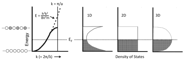
Density of States (DOS)
- The density of states is defined as the number of orbitals per unit of energy within a band.
- Because of the parabolic relation between \(E\) and \(k\), the density of states for a 1D metallic crystal is highest near the bottom and top of the energy band where the slope of the \(E\) vs. \(k\) curve is closest to zero.
- The shape of the DOS curve is different in crystals of higher dimensionality as shown in the figure in the left, because statistically there are more ways to make an orbital with \(\frac{N}{2}\) nodes than there are with zero or \(N\) nodes.
- The situtation is analogous to the numbers you can make by rolling dice. With one die, the numbers 1-6 have equal probability. However, with two dice there is only one way to make a two (snake eyes) or a twelve (boxcars), but many ways to make a seven.
Single-Walled Carbon Nanotubes
- While most of the time we will talk about 3D crystals that have their maximum DOS near the middle of the energy band, there are examples of quasi-1D systems, such as carbon nanotubes.
- Metallic carbon nanotubes have strong optical absorption bands that correspond to transitions between the two regions of high DOS (the van Hove singularities) near the bottom and top of the bands.
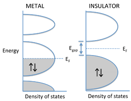
Metals, Semiconductors, and Insulators
- The degree to which bands fill determines whether a crystalline solid is a metal, semiconductor, or insulator.
- If the highest occupied molecular orbitals lie within a band - i.e., if the Fermi level EF cuts through a band of orbitals - then the electrons are free to change their speed and direction in an electric field and the solid is metallic.
- However, if the solid contains just enough electrons to completely fill a band, and the next highest set of molecular orbitals is empty, then it is a semiconductor or insulator.
- In this case, there is an energy gap between the filled and empty bands, which are called the valence and conduction bands, respectively.
Example
Band Gaps
- Although the distinction is somewhat arbitrary, materials with a large gap (\( \gt 3\, eV\)) are called insulators
- Those with smaller gaps are called semiconductors.
- We will learn more about the properties of semiconductors later.
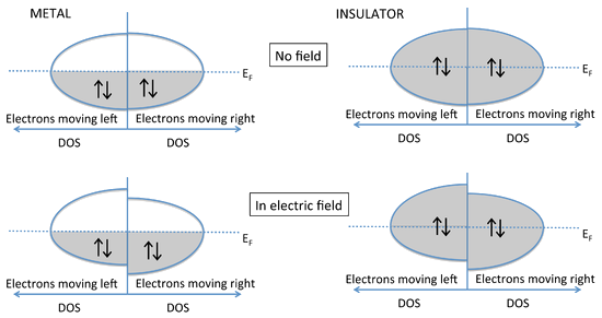
Why Don't Insulators Conduct Electricity?
- The energy vs. DOS diagram shows what happens when an electric field is applied to a metal or an insulator.
- The diagram to shows explicitly the energies of electrons moving left and right.
- These energies are the same in the absence of an electric field.
- Once we apply a field (e.g., by putting a voltage across a metal wire), the electrons moving in the direction of the field have lower energy than those moving in the opposite direction.
Why Don't Insulators Conduct Electricity?
- In the case of the metal, the populations of electrons moving with and against the electric field are different, and there is a net flow of current.
- Note that this can happen only when the Fermi level cuts through a partially filled band.
- With a semiconductor or insulator, the valence band is filled and the conduction band is empty.
- Thus, applying an electric field changes the energies of electrons traveling with and against the field, but because the band is filled, the same number are going in both directions and there is no net current flow.
Conduction in Metals
- In metals, the valence electrons are in molecular orbitals that extend over the entire crystal lattice.
- Metals are almost always crystalline and the individual crystal grains are typically micron size.
- Thus, the spatial extent of the orbitals is very large compared to the size of the atoms or the unit cell.
- In some cases, there are \(N\) orbitals for \(N\) electrons, and each orbital can accomodate two electrons.
- The Fermi level, which corresponds to the energy of the highest occupied MO at zero temperature, is somewhere in the middle of the band of orbitals.
- The energy level spacing between orbitals is very small compared to the thermal energy \(kT\), so we can think of the orbitals as forming a continuous band.
Specific Heat Paradox
- Classically, if the electrons in this band were free to be thermally excited, we would expect them to have a specific heat of \(3R\) per mole of electrons.
- However, experimentally we observe that \(C_p\) is only about \(0.02 R\) per mole.
- This suggests that only about 1% of the electrons in the metal can be thermally excited at room temperature.
- However, essentially all of the valence electrons are free to move in the crystal and contribute to electrical conduction.
Specific Heat Paradox Solution
- This paradox is solved by recalling that the electrons exist in quantized energy levels.
- Because of quantization, electrons in metals have a Fermi-Dirac distribution of energies.
- In this distribution, most of the electrons are spin-paired, although the individual electrons in these pairs can be quite far apart since the orbitals extend over the entire crystal.
- A relatively small number of electrons at the top of the Fermi sea are unpaired by thermal excitation.
- This is the origin of the Pauli paramagnetism of metals.
Let's look more closely.
- Because of the bell shape of the \(E\) vs. DOS curve, most of the electrons have \(E \approx E_F\).
- At the midpoint energy (\(E_F\)) of the band, the MO's have one node for every two atoms.
- We can calculate the de Broglie wavelength as twice the distance between nodes and thus \(\lambda = 4a\) at the midpoint of the band, where \(a\) is the interatomic spacing.
- Since a typical value of \(a\) is about \(2\, \AA\), we obtain the de Broglie wavelength \(\lambda \approx 8\AA\).
- Using the de Broglie relation \(p = \frac{h}{\lambda}\), we can say \(p=h\lambda = m_e v_F\) where
- \(m_e\) is the mass of the electron
- \(v_F\) is the velocity of electrons with energy \(E_F\)
How fast are electrons traveling in a typical metal?
- Solving for \(v_F = \frac{h}{m_e\lambda}\) we obtain \(v_F = \frac{6.62\times 10^{-34}J\cdot s}{(9.1\times 10^{-31}kg)(8\times 10^{-10}m)}=1.0\times 10^6\frac{m}{s}\)
- Experimental values of \(v_F\) are \(1.07 \times 10^6\) and \(1.39 \times 10^6 \frac{m}{s}\) for Na and Ag, respectively, so our approximations are pretty good.
- So how fast are electrons moving in metals? Really, really fast!! 1,000,000 meters per second!
- This is about 1/300 the speed of light, and about 3000 times the speed of sound (\(3 \times 10^2 m/s\)).
Drift Velocity
- The drift velocity of electrons in metals is quite slow, on the order of \(0.0001\frac{m}{s}\), or \(0.01 \frac{cm}{s}\).
- You can easily outrun an electron drifting in a metal, even if you have been drinking all night and have been personally reduced to a very slow crawl.
The Differences in the Velocities
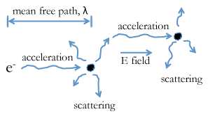
- Why the great disparity between the Fermi velocity and the drift velocity of electrons in metals?
- We need to consider a picture for the scattering of electrons, and their acceleration in an electric field, as shown on the previous slide.
- If we apply a voltage across a metal (e.g., a metal wire), the electrons are subjected to an electric field \(E\), which is the voltage divided by the length of the wire.
- This electric field exerts a force on the electron, causing it to accelerate.
Electron Scattering
- However, the electron is frequently scattered, mostly by phonons (lattice vibrations).
- Each time the electron is scattered its acceleration starts all over again.
- The time between scattering events is \(\tau\) and the distance the electrons travel between scattering events is the mean free path, \(\lambda\), which is functionally akin the concept by the same name in kinetic molecular theory.
The Force on the Electron
- We can write the force on the electron as:
\[ F=eE=m_ea=\frac{m_e v_{drift}}{\tau} \]
where
- \(a\) is the acceleration in the electric field
- \(m_e\) is the mass
- \(v_{drift}\) is the drift velocity of the electron
The Mean Free Path of the Electron
- Experimentally, the mean free path is typically obtained by measuring the scattering time.
- For an electron in Cu metal at 300 K, the scattering time \(\tau\) is about \(2 \times 10^{-14} s\).
- From this we can calculate the mean free path as:
\[ \lambda = v_{avg}\tau \approx v_F\tau =(1\times 10^6\frac{m}{s})(2\times 10^{-14}s)=40\, nm \]
- The mean free path (\(40 nm = 400 \AA\)) is quite long compared to the interatomic spacing (\(2 \AA\)).
- To put it in perspective, if the interatomic spacing was scaled to the length of a football (0.3 m), the mean free path would be over half the length of the football field (60 m).
Interesting Connection
- So, electrons are traveling in metals at the Fermi velocity \(v_F\), which is very, very fast (\(10^6 \frac{m}{s}\)), but the flux of electrons is the same in all directions.
- In an electric field, a very small but directional drift velocity is superimposed on this fast random motion of valence electrons.
- An important consequence of this calculation is Ohm's Law, \(V=IR\)
- From the equations above, we can see that the drift velocity increases linearly with the applied electric field \(v_{drift}=a\tau = \frac{eE\tau}{m_e}\)
- The drift velocity is proportional to the current, and the electric field is proportional to the voltage.
- So, \(V = IR\), where \(R\) is the combination of the two proportionality constants.
Electrical Conductivity
- The conductivity (\(\sigma\)) of a metal is proportional to \(\tau\) (and \(\lambda\))
\[ \sigma = \frac{ne^2 \tau}{m_e} \]
where \(n\) is the density of valence electrons (\(8.5 \times 10^{28} m^{-3}\) for Cu) and \(e\) is the electronic charge.
- Putting in the numbers and converting to \(cm\) units we obtain \(\sigma = 7 \times 10^5 \Omega^{-1}cm^{-1}\) for Cu, in good agreement with the measured value (\(6 \times 10^5 \Omega^{-1}cm^{-1}\)).
Atomic Orbitals and Magnetism
- Can MO theory help us rationalize the electrical conductivity of Mg with its \(3s^2\)?
- The two valence electrons are spin-paired in atomic Mg, as they are in the helium atom (\(1s^2\)).
- When the \(3s\) orbitals of Mg combine to form a band, we would expect the band to be completely filled, since Mg has two electrons per orbital.
- By this reasoning, solid Mg should be an insulator.
- But Mg has all the properties of a metal: high electrical and thermal conductivity, metallic luster, malleability, etc.
What's going on with Mg?
![The cohesive energy of Mg metal is the difference between the bonding and promotion energies. The ground state of a gas phase Mg atom is [Ar]3s2, but it can be promoted to the [Ar]3s13p1 state, which is 264 kJ/mol above the ground state. Mg uses two electrons per atom to make bonds, and the sublimation energy of the metal is 146 kJ/mol.](./figures/MetalsAndAlloys/Mg_promotion.png)
- In this case the \(3s\) and \(3p\) bands are sufficiently broad (because of strong orbital overlap between Mg atoms) that they form a continuous band.
- This band, which contains a total of four orbitals (one \(3s\) and three \(3p\)) per atom, is only partially filled by the two valence electrons.
- Alternatively, consider hybridization.
- Hybridization requires promotion from the \(3s^23p^0\) ground state of an Mg atom to a \(3s^13p^1\) excited state.
- The promotion energy (+264 kJ/mol) is more than offset by the bonding energy (-410 kJ/mol)
Heats of Vaporization
- The heat of vaporization, or the cohesive energy of a metal, is the difference between the bonding energy and the promotion energy.
- Experimentally, we can measure the vaporization energy (+146 kJ/mol) and the promotion energy and use them to calculate the bonding energy.
- From this we learn that each s or p electron is worth about 200 kJ/mol in bonding energy.
- The concepts of promotion energy and bonding energy are very useful in rationalizing periodic trends in the bond strengths and magnetic properties of metals
Periodic Trends in d-Electron Bonding
- While electrons in \(s\) and \(p\) orbitals tend to form strong bonds, d-electron bonds can be strong or weak.
- There are two important periodic trends that are related to orbital size and orbital overlap.
- As we move across the periodic table (Sc - Ti - V - Cr - Fe), the d orbitals contract because of increasing nuclear charge.
- Moving down the periodic table (V - Nb - Ta), the d orbitals expand because of the increase in principal quantum number.
- In the 3d series, the contraction of orbitals affects the ability of the d electrons to contribute to bonding.
- Past V in the first row of the transition metals, the 3d electrons become much less effective in bonding because they overlap weakly with their neighbors.
- Weak overlap of 3d orbitals gives narrow d-bands and results in the emergence of magnetic properties.
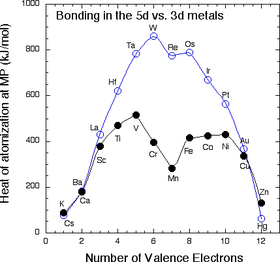
Work and Heat
- In the 4d and 5d series, a plot of cohesive energy vs. number of valence electrons has a "volcano" shape that is peaked at the elements Mo and W (5s14d5 and 6s15d5, respectively).
- The number of bonding electrons, and therefore the bonding energy, increases steadily going from Rb to Mo in the 4d series, and from Cs to W in the 5d series.
- Mo and W have the most bonding energy because they can use all six of their valence electrons in bonding without promotion.
Work and Heat
- Elements past Mo and W have more d electrons, but some of them are spin paired and so some promotion energy is needed to prepare these electrons for bonding.
- Because of their strong bonding energy, elements in the middle of the 4d and 5d series have very high melting points.
- We do not see magnetism in the 4d or 5d metals or their alloys because orbital overlap is strong and the bonding energy exceeds the electron pairing energy.
The \(3d\) Elements
- The 3d elements (Sc through Zn) are distinctly different from the 4d and 5d elements in their bonding (and consequently in their magnetic properties).
- In the 3d series, we see the expected increase in cohesive energy going from Ca (\(4s^2\)) to Sc (\(4s^23d^1\)) to Ti (\(4s^23d^2\)) to V (\(4s^23d^3\))
- As we have seen, the 3d series has a "crater" in the cohesive energy plot where there was a peak in the 5d series.
- The cohesive energy actually decreases going from V to Mn, even though the number of valence electrons is increasing.
- We can explain this effect by remembering that the 3d orbitals are progressively contracting as more protons are added to the nucleus.
The \(3d\) Elements Beyond V
- For elements beyond V, the orbital overlap is so poor that the 3d electrons are no longer effective in bonding, and the valence electrons begin to unpair.
- At this point the elements become magnetic.
- Depending on the way the spins order, metals and alloys in this part of the periodic table can be ferromagnetic (spins on neighboring atoms aligned parallel, as in the case of Fe or Ni) or antiferromagnetic (spins on neighboring atoms antiparallel, as in the case of Mn).
- At short interatomic distances (or with strong overlap between atomic orbitals), the spins of the electrons pair and a bond is formed.
- Unpairing the electrons becomes favorable at larger interatomic distances where the overlap between orbitals is poor.
Alloys of the 4f Elements
- Many alloys of the 4f elements (the lanthanides) are also magnetic because the 4f orbitals, like the 3d orbitals, are poorly shielded from the nuclear charge and are ineffective in bonding.
- Strong permanent magnets often contain alloys of Nd, Sm, or Y, usually with magnetic 3d elements such as Fe and Co.
- Because the 4f orbitals are contracted and not very effective in bonding, other physical properties of the lanthanides are also affected.
- For example, oxides of the 4f elements have rather weak surface interactions with polar molecules such as water.
- Consequently, oxides such as \(CeO_2\), \(Er_2O_3\), and \(Ho_2O_3\) are hydrophobic, whereas main group and early transition metal oxides (e.g., \(Al_2O_3\), \(SiO_2\), \(TiO_2\)) are quite hydrophilic.
Late Transition Metal Alloys
- Although the bonding in the 5d series follows a "normal" volcano plot, the situation is a bit more complex for alloys of Re, Os, Ir, Pt, and Au.
- There is strong overlap between the 5d orbitals, but because these elements contain more than five d-electrons per atom, they cannot make as many bonds as 4d or 5d elements with half-filled d-shells such as Mo or W.
- This progressive filling of the d-band explains the steady decrease in bonding energy going from Os to Au.
- Pt and Au are both soft metals with relatively low heats of vaporization.
- However, these metals (especially Ir, Pt, and Au) can combine with early transition metals to form stable alloys with very negative heats of formation and high melting points.
- For example, ZrC and Pt react to form a number of stable alloys (\(ZrPt\), \(Zr_9Pt_{11}\), \(Zr_3Pt_4\), \(ZrPt_3\)) plus carbon.
More on Late Transition Metal Alloys
- This reactivity is unusual because we normally think of Pt as a "noble" (i.e., unreactive) metal, and because ZrC is a very stable, refractory metal carbide.
- The favorable combination of early and late transition metals has been interpreted as arising from a d-electron "acid-base" interaction.
- For example, in \(HfPt_3\), Hf is the "acid" with an electron configuration of \(6s^25d^2\), while Pt is the "base" with the electron configuration of \(6s^15d^9\).
- They combine to create a stable "salt" product with a filled 5d electron configuration without promoting any electrons to higher orbitals.
- The implication is that Pt donates d-electrons to the "d-acid," Zr or Hf.
- However, electronic structure calculations on model compounds show that much of the bonding energy in \(ZrPt\) and \(ZrPt_3\) arises from electron transfer from Zr to Pt (not the other way around) and the polarity of the resulting metal-metal bonds.
Even More on Late Transition Metal Alloys
- Regardless of the source of their stability, some early-late transition metal alloys are of particular interest for use in catalysis.
- For example, the alloy \(ScPt_3\) is a good catalyst for oxygen reduction in fuel cells.
- Even though Sc is an active metal that is, it is stabilized in the aqueous acid environment of the fuel cell by its strong interaction with Pt.
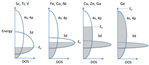
Filling of the \(3d\) and \(4s\), \(4p\) Bands
- In the 3d series, we see magnetic behavior for elements and alloys between Cr and Ni.
- Past Ni, the elements (Cu, Zn, Ga,...) are no longer magnetic and they are very good electrical conductors, implying that their valence electrons are highly delocalized.
- We can understand this behavior by considering the overlap of 4s, 4p, and 3d orbitals, all of which are close in energy.
- The 4s and 4p have strong overlap and form a broad, continuous band.
- On the other hand, the 3d electrons are contracted and form a relatively narrow band.
- Progressing from the early 3d elements (Sc, Ti, V), we begin to fill the 3d orbitals, which are not yet so contracted that they cannot contribute to bonding.
- Thus, the valence electrons in Sc, Ti, and V are all spin-paired, except for a small number near the Fermi level that give rise to a weak Pauli paramagnetism.
Continuing Acrros the Rows
- Moving across the 3d series to the magnetic elements (Fe, Co, Ni), the d-orbitals are now so contracted that their electrons unpair and we see cooperative ordering of spins (ferromagnetism and antiferromagnetism).
- Referring to the band diagram at the right, the 3d band is only partially filled and the Fermi level cuts through it.
- For Cu, Zn, and Ga, the 3d orbitals are even more contracted and the 3d band is thus more narrow, but now it is completely filled and the Fermi level is in the 4s,4p band.
- The strong orbital overlap in these bands results in spin pairing and a high degree of electron delocalization.
- Consequently, metals in this part of the periodic table (Cu, Ag) are diamagnetic and are among the best electrical conductors at room temperature.
- Finally, at Ge, the 4s,4p band is completely filled and the solid is a semiconductor.
Some Magnetic Behavior
- Materials are classified as diamagnetic if they contain no unpaired electrons.
- Diamagnetic substances are very weakly repelled from an inhomogeneous magnetic field.
- Molecules or ions that have unpaired spins are paramagnetic and are attracted to a magnet, i.e., they move towards the high field region of an inhomogeneous field.
- This attractive force results from the alignment of spins with the field, but in the case of paramagnetism each molecule acts independently.
- In metals, alloys, oxides, and other solid state compounds, the unpaired spins interact strongly with each other and can order spontaneously, resulting in the cooperative magnetic phenomena described below.
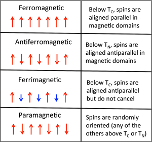
Ferro-, Ferri-, and Antiferromagnetism
The magnetism of metals and other materials are determined by the orbital and spin motions of the unpaired electrons and the way in which unpaired electrons align with each other.
All magnetic substances are paramagnetic at sufficiently high temperature, where the thermal energy (\(kT\)) exceeds the interaction energy between spins on neighboring atoms.
Below a certain critical temperature, spins can adopt different kinds of ordered arrangements.
Ordering of Spins
Iron
- Fe is in group VIIIb of the periodic table, so it has eight valence electrons.
- The atom is promoted to the \(4s^13d^7\) state in order to make bonds. A localized picture of the d-electrons for an individual iron atom might look like this:
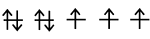
- The total spin angular momentum, \(S\), for this atom is: \( S=3\left( \frac{1}{2}\right)=\frac{3}{2}\)
- We can think of each Fe atom in the solid as a little bar magnet with a spin-only moment \(S\) of \(\frac{3}{2}\).
- The spin moments of neigboring atoms can align in parallel (\(\uparrow \uparrow\)), antiparallel (\(\uparrow \downarrow\)), or random fashion.
- In bcc Fe, the tendency is to align parallel because of the positive sign of the exchange interaction.
- This results in ferromagnetic ordering, in which all the spins within a magnetic domain (typically hundreds of unit cells in width) have the same orientation.
Other Metals
- Conversely, a negative exchange interaction between neighboring atoms in bcc Cr results in antiferromagnetic ordering.
- A third arrangement,ferrimagnetic ordering, results from an antiparallel alignment of spins on neighboring atoms when the magnetic moments of the neighbors are unequal.
- In this case, the spin moments do not cancel and their is a net magnetization.
- The ordering mechanism is like that of an antiferromagnetic solid, but the magnetic properties resemble those of a ferromagnet.
- Ferrimagnetic ordering is most common in metal oxides
Magnetization and Susceptibility
- The magnetic susceptibility, \(\chi\), of a solid depends on the ordering of spins.
- Paramagnetic, ferromagnetic, antiferromagnetic, and ferrimagnetic solids all have \(\chi \gt 0\), but the magnitudes of their susceptibility varies with the kind of ordering and with temperature.
- We will see these kinds of magnetic ordering primarily among the 3d and 4f elements and their alloys and compounds.
- For example, \(Fe\), \(Co\), \(Ni\), \(Nd_2Fe_{14}B\), \(SmCo_5\), and \(YCo_5\) are all ferromagnets, \(Cr\) and \(MnO\) are antiferromagnets, and \(Fe_3O_4\) and \(CoFe_2O_4\) are ferrimagnets.
- Diamagnetic compounds have a weak negative susceptibility (\(\chi \lt 0\)).
Susceptibility of Paramagnets
- For a paramagnetic substance, \( \chi^{corr}_M=\frac{C}{T} \)
- The inverse relationship between the magnetic susceptibility and \(T\), the absolute temperature, is called Curie's Law, and the proportionality constant \(C\) is the Curie constant: \( C=\frac{N_A}{3k_B}\mu_{eff}^2 \)
- Note that \(C\) is not a "constant" in the usual sense, because it depends on \(\mu_{eff}\), the effective magnetic moment of the molecule or ion, which in turn depends on its number of unpaired electrons: \( \mu_{eff}=\sqrt{n(n+2)}\mu_B \)
- Here \(\mu_B\) is the Bohr magneton, a physical constant defined as \(\mu_B = \frac{eh}{4\pi m_e} = 9.274 \times 10^{-21} \frac{erg}{gauss}\) (in cgs units).
Simplicication
- In cgs units, we can combine physical constants, \( \frac{N_A}{3k_B}\mu_B^2=0.125\)
- Combining these equations, we obtain \(\chi_M^{corr}=\frac{0.125}{T}\left( \frac{\mu_{eff}}{\mu_B} \right)^2\)
- These equations relate the molar susceptibility, a bulk quantity that can be measured with a magnetometer, to \(\mu_{eff}\), a quantity that can be calculated from the number of unpaired electrons, \(n\).
- Two important points to note about this formula are:
- The magnetic susceptibility is inversely proportional to the absolute temperature, with a proportionality constant \(C\) (Curie's Law)
- So far we are talking only about paramagnetic substances, where there is no interaction between neighboring atoms.
Plotting the Curie Constant
- The plot below shows the number of unpaired electrons per atom, calculated from measured Curie constants, for the magnetic elements and 1:1 alloys in the 3d series.
- The plot peaks at a value of 2.4 spins per atom, slightly lower than we calculated for an isolated iron atom.
- This reflects that fact that there is some pairing of d-electrons, i.e., that they do contribute somewhat to bonding in this part of the periodic table.
.png)
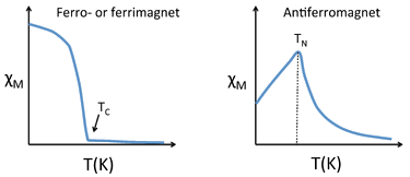
Susceptibility of Ferro-, Ferri-, and Antiferromagnets
- Below a certain critical temperature, the spins of a solid paramagnetic substance order and the susceptibility deviates from simple Curie-law behavior.
- Because the ordering depends on the short-range exchange interaction, this critical temperature varies widely.
- Metals and alloys in the 3d series tend to have high critical temperatures because the atoms are directly bonded to each other and the interaction is strong.
- For example, Fe and Co have critical temperatures (also called the Curie temperature, \(T_c\), for ferromagnetic substances) of \(1043\) and \(1400\, K\), respectively.
- The Curie temperature is determined by the strength of the magnetic exchange interaction and by the number of unpaired electrons per atom.
- The number of unpaired electrons peaks between Fe and Co as the d-band is filled, and the exchange interaction is stronger for Co than for Fe.
- In contrast to ferromagnetic metals and alloys, paramagnetic salts of transition metal ions typically have critical temperatures below \(1\, K\) because the magnetic ions are very weakly coupled electronically.
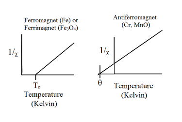
Curie-Weiss Law
- Above the critical temperature \(T_C\), ferromagnetic compounds become paramagnetic and obey the Curie-Weiss law: \( \chi = \frac{C}{T-T_C} \)
- This is similar to the Curie law, except that the plot of \(\frac{1}{\chi}\) vs. \(T\) is shifted to a positive intercept \(T_C\) on the temperature axis.
- This reflects the fact that ferromagnetic materials (in their paramagnetic state) have a greater tendency for its spins to align in a magnetic field than an ordinary paramagnet in which the spins do not interact with each other.
- Ferrimagnets follow the same kind of ordering behavior.
Typical Plots for Ferro- and Ferrimagnets
Antiferromagnets
- Antiferromagnetic solids are also paramagnetic above a critical temperature, which is called the Néel temperature, \(T_N\).
- For antiferromagnets, \(\chi\) reaches a maximum at \(T_N\) and is smaller at higher temperature (where the paramagnetic spins are further disordered by thermal energy) and at lower temperature (where the spins pair up).
- Typically, antiferromagnets retain some positive susceptibility even at very low temperature because of canting of their paired spins.
- However the maximum value of \(\chi\) is much lower for an antiferromagnet than it is for a ferro- or ferrimagnet.
- The Curie-Weiss law is also modified for an antiferromagnet, reflecting the tendency of spins (in the paramagnetic state above \(T_N\)) to resist parallel ordering.
- A plot of \(\frac{1}{\chi}\) vs. \(T\) intercepts the temperature axis at a negative temperature, \(-\theta\), and the Curie-Weiss law becomes: \( \chi =\frac{C}{T+\theta} \)
Ordering of Spins Below \(T_C\)
- Below \(T_C\), the spins align spontaneously in ferro- and ferrimagnets.
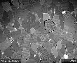
- Complex magnetization behavior is observed that depends on the history of the sample. For example, if a ferromagnetic material is cooled in the absence of an applied magnetic field, it forms a mosaic structure of magnetic domains that each have internally aligned spins.
- However, neighboring domains tend to align the opposite way in order to minimize the total energy of the system.
- This is illustrated in the figure on the following slide for a Nd-Fe-B magnet.
- The sample consists of \( 5-10\,\mu m\) wide crystal grains that can be easily distinguished by the sharp boundaries in the image.
- Within each grain are a series of lighter and darker stripes (imaged by using the optical Kerr effect) that are ferromagnetic domains with opposite orientations.
- Averaged over the whole sample, these domains have random orientation so the net magnetization is zero.
Nd-Fe-B Magnet
Appling a Magnetic Field
- When a sample like this one is magnetized (i.e., exposed to a strong magnetic field), the domain walls move and the favorably aligned domains grow at the expense of those with the opposite orientation.
- This transformation can be seen in real time in the Kerr microscope.
- The domain walls are typically hundreds of atoms wide, so movement of a domain wall involves a cooperative tilting of spin orientation (analogous to "the wave" in a sports stadium) and is a relatively low energy process.

Magnetization
- The process of magnetization moves the solid away from its lowest energy state (random domain orientation), so magnetization involves input of energy.
- When the external magnetic field is removed, the domain walls relax somewhat, but the solid (especially in the case of a "hard" magnet) can retain much of its magnetization.
- If you have ever magnetized a nail or a paper clip by using a permanent magnet, what you were doing was moving the walls of the magnetic domains inside the ferromagnet.
- The object thereafter retains the "memory" of its magnetization.
- However, annealing a permanent magnet destroys the magnetization by returning the system to its lowest energy state in which all the magnetic domains cancel each other.
Magnetic Hysteresis
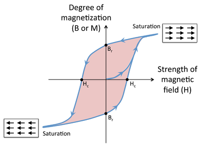
- Cycling a ferro- or ferrimagnetic material in a magnetic field results in hysteresis in the magnetization of the material, as shown in the figure below.
- At the beginning, the magnetization is zero, but it begins to rise rapidly as the magnetic field is applied.
- At high field, the magnetic domains are aligned and the magnetization is said to be saturated.
- When the field is removed, a certain remanent magnetization (indicated as the point \(B_r\) on the graph) is retained, i.e., the material is magnetized.
Magnetic Hysteresis Continued
- Applying a field in the opposite direction begins to orient the magnetic domains in the other direction, and at a field \(H_c\) (the coercive field), the magnetization of the sample is reduced to zero.
- Eventually the material reaches saturation in the opposite direction, and when the field is removed again, it has remanent magnetization \(B_r\), but in the opposite direction.
- As the field continues to reverse, the magnet follows the hysteresis loop as indicated by the arrows.
- The area of colored region inside the loop is proportional to the magnetic work done in each cycle.
- When the field cycles rapidly (for example, in the core of a transformer, or in read-write cycles of a magnetic disk) this work is turned into heat.
Hard and Soft Magnets
- Whether a ferro- or ferrimagnetic material is a hard or a soft magnet depends on the strength of the magnetic field needed to align the magnetic domains.
- This property is characterized by \(H_c\), the coercivity.
- Hard magnets have a high coercivity (\(H_c\)), and thus retain their magnetization in the absence of an applied field, whereas soft magnets have low values.
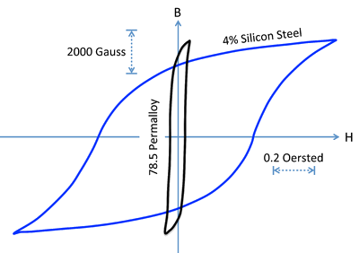
Compring Hysteresis Loops
- The figure below compares hysteresis loops for hard and soft magnets.
- Recall that the energy dissipated in magnetizing and demagnetizing the material is proportional to the area of the hysteresis loop.
- We can see that soft magnets, while they can achieve a high value of \(B_{sat}\), dissipate relatively little energy in the loop.
- This makes soft magnets preferable for use in transformer cores, where the field is switched rapidly.
- Permalloy, an alloy consisting of about 20% Fe and 80% Ni, is a soft magnet that has very high magnetic permeability \(\mu\) (i.e., a large maximum slope of the \(B\) vs. \(H\) curve) and a very narrow hysteresis loop.
Both Hard and Soft
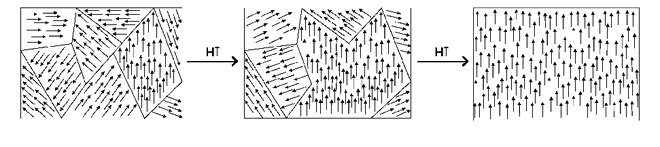
- Some materials, such as iron metal, can exist as either hard or soft magnets.
- Whether bcc iron is a hard or soft magnet depends on the crystal grain size.
- When crystal grains in iron are sub-micron size, and comparable to the size of the magnetic domains, then the magnetic domains are pinned by crystal grain boundaries.
- When the magnetic domains are pinned a stronger coercive magnetic field needs to be applied to cause them to re-align.
- When iron is annealed, the crystal grains grow and the magnetic domains become more free to align with applied magnetic fields.
- This decreases the coercive field and the material becomes a soft magnet.
Hard Magnets
- Hard magnets such as \(CrO_2\), \(\gamma-Fe_2O_3\), and cobalt ferrite (\(CoFe_2O_4\)) are used in magnetic recording media, where the high coercivity allows them to retain the magnetization state (read as a logical 0 or 1) of a magnetic bit over long periods of time.
- Hard magnets are also used in disk drives, refrigerator magnets, electric motors and other applications.
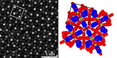
- Drive motors for hybrid and electric vehicles such as the Toyota Prius use the hard magnet \(Nd_2Fe_{14}B\) (also used to make strong refrigerator magnets) and require 1 kilogram (2.2 pounds) of neodymium.
- A high-resolution transmission electron microscope image of \(Nd_2Fe_{14}B\) is shown below and compared to the crystal structure with the unit cell marked.
/