Indroduction to Statistical Mechanics: Building Up to the Bulk

Shaun Williams, PhD

Atomic Structure

Atomic Structure

• A concept key to interpreting the second law of thermodynamics is the limitation by quantum mechanics on the number of states of our system
  • The number of quantum states of any real system is a finite number
• This is an important difference between our classical understanding and our modern understanding

Quantization of Properties

• At molecular sizes, particles behave like waves
• To fulfill the mathematical rules of waves, parameters, such as energy and momentum, are only allowed certain quantized values
• For a moving particle particle, this quantization becomes measurable when the distance traveled is much greater than its de Broglie wavelength $$ \lambda_{dB} = \frac{h}{mv} $$
• In this equation, called the de Broglie wavelength equation
  • \(h\) is Planck’s constant, \( 6.626 \times 10^{-34}\,\mathrm{J}\cdot \mathrm{s}\)
  • \(m\) is the particles mass
  • \(v\) is the particles velocity

Quantizer Energy

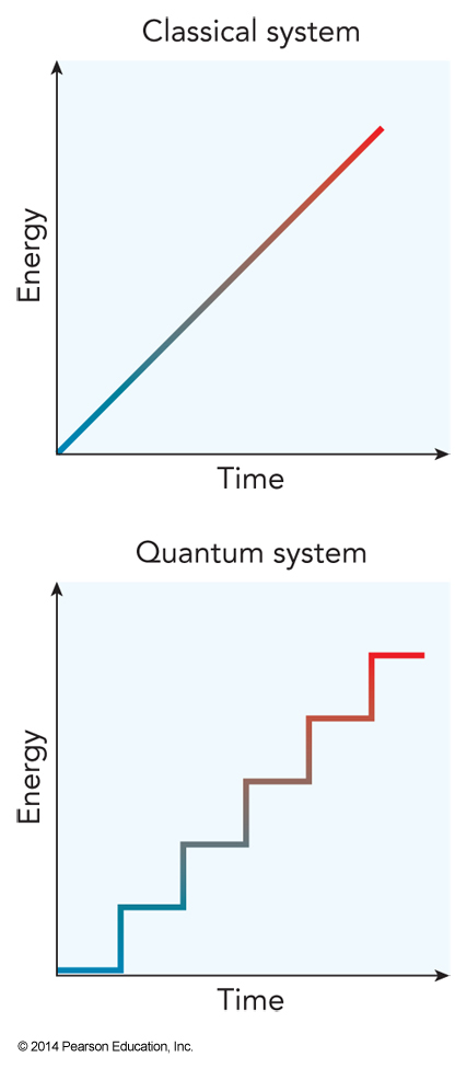
• In a classical system, energy is a continuous function
• In a quantum system, energy comes only in discrete values

Problem with the quantum nature

• When dealing with waves, the particles/waves cannot have their position pinned down to a single location
• For any parameter, \(A\left(\vec{r}\right)\), the average value of this parameter is given by the average value theorem $$ \expect{A} = \int_{\text{all space}} \mathcal{P}_\vec{r}\left(\vec{r}\right) A\left(\vec{r}\right) d\vec{r} $$
  • Where \(\mathcal{P}_\vec{r}\left(\vec{r}\right)\) is the probability distribution

Particle in a Three-Dimensional Box

• Consider a 3-D box with lengths of \(a\), \(b\), and \(c\) along the \(x\), \(y\), and \(z\) axes, respectively
• Possible energy values for a particle in the box is $$ \begin{align} \varepsilon_{n_x,n_y,n_z} &= \frac{\pi^2 \hbar^2}{2m}\left( \frac{n_x^2}{a^2}+\frac{n_y^2}{b^2}+\frac{n_z^2}{c^2} \right) \\ &\approx \frac{\pi^2\hbar^2}{2m(abc)^\bfrac{2}{3}}\left( n_x^2+n_y^2+n_z^2 \right) = \varepsilon_0n^2 \end{align} $$

Energy Levels of a Three-Dimensional Box

States of Such a Particle

• A particle which has the lowest values of \(n_x\), \(n_y\) and \(n_z\) is said to be in its ground state
  • Any other state is said to an excited state
• When two or more quantum states share the same energy, we say they are degenerate
  • (2,1,1), (1,2,1), and (1,1,2)
• Correspondence principle – quantum mechanics approaches classical mechanics as we increase the particle’s kinetic energy, mass, or domain

Use of Quantum Mechanics

• Due to correspondence principle:
  • Use QM when \(\lambda_{dB}\) is comparable to the domain size
  • Use classical when \(\lambda_{dB}\) is much smaller
• Entropy allows us to indirectly measure the density of quantum states, \(W(\varepsilon)\)
• The density of states tells how many quantum states near energy \(\varepsilon\) there are per unit energy

Quantum States of Atoms

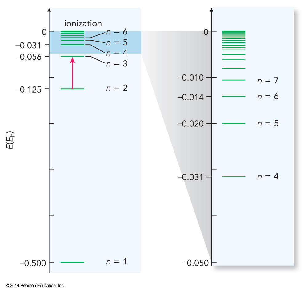
• The same analysis can be used on one-electron atoms yielding $$ E_n = -\frac{Z^2m_ee^4}{2\left(4\pi \epsilon_0\right)^2n^2\hbar^2} \equiv -\frac{Z^2}{2n^2}E_h $$
• \(E_h\) is the energy unit Hartree
• Hartrees are convenient units for calculations involving electrons in atoms
• Conversion: \(1\,E_h=4.360\times 10^{-18}\,\mathrm{J}\)

Energy Levels of the Hydrogen Atom

Quantum State of Electrons

• The quantum state of electrons depend on three other quantum numbers
  • \(l\) – angular momentum quantum number; defines the shape
  • \(m_l\) – magnetic quantum number; defines orientation in space
  • \(m_s\) – spin angular momentum
• For each atom, we can specify the entire set of quantum numbers (electron configuration)

Term Symbols

• In addition to electron configurations, which give \(n\) and \(l\) values, we can specify the term symbol which gives \(m_l\) and \(m_s\) values
  • Ground state of nitrogen is \( 1s^22s^22p^3\) and it has a term symbol of \({}^4S\)

Electron Spin

• Spin is really an intrinsic property, like mass and charge
• Particles called Fermions all have spins that are half-integers
  • Electrons, protons, neutrons
• Particles called Bosons all have integer spins
  • \(\chem{{}^4He}\) nucleus

The Pauli Exclusion Principle

• No two individual Fermions can have the same set of quantum numbers
• Unlike Fermions, according to the Pauli exclusion principle, multiple Bosons can have the same set of quantum numbers
  • This gives rise to very interesting effects (chapter 4)

Degrees of Freedom

• Atoms in molecules attract and repel.
• Energy added to a molecule goes into one of 4 forms of motion
  • Electronic – fast motion
  • Vibrational
  • Rotational
  • Translational – slow motion
• Note: increasing mass of the moving particle

Translational Energy

• Due to its large mass and slow speed, translational energy can normally be treated classically $$ K=\frac{mv^2}{2} $$
• We don’t need to worry too much about the other forms yet
• When energy is added to a system, it distributes itself into some or all of these degrees of freedom

Electronic State Transitions (UV-vis)

• Quantum states of molecules is not so easy
• Exciting from the electronic ground state to excited state gives us information
• This is done with electromagnetic (EM) radiation
• A photon has energy given by Planck’s law $$ E_{photon} = h\nu = \frac{hc}{\lambda} $$
  • \(c\) – speed of light: \(c=2.9979\times 10^8\,\mathrm{m}\,\mathrm{s}^{-1}\)

Vibrational State Transitions (IR)

• After electronic, the remaining contributions come from the motion of the nuclei
• For \(N_{atom}\) in the molecule, there are a total of \(3N_{atom}\) degrees of freedom
• Number of vibrational degrees of freedom:
  • For non-linear molecules: \(3N_{atom}-6\)
  • For linear molecules: \(3N_{atom}-5\)

Vibrational Modes

• For each vibrational coordinate we can define a vibrational constant, \(\omega_e\)
  • Depends on mass of atoms and rigidity of bond
• Harmonic approximation defined the constant $$ \omega_e(J)=\hbar \sqrt{\frac{k}{\mu}} $$
  • The reduced mass is \(\mu=\frac{m_Am_B}{m_A+m_B}\)

Vibrational Energies

• The quantum states for vibrational motion have vibrational energies approximately equal to $$ E_v=\left(v+\frac{1}{2}\right)\omega_e $$
  • \(v\) can be any integer 0 or greater
• Vibrational energies correspond to the infrared region of the EM spectrum

Rotational States Transions (microwave)

• Non-linear molecules have three rotational coordinates
• Linear molecules have two rotational coordinates
• For a simple linear molecule the rotational energies are given by $$ E_J=BJ(J+1) $$
  • \(B\) is the rotational constant
  • \(J\) can be any integer 0 or greater

Rotational State Degeneracies

• Rotational states have degeneracies corresponding to different orientations of rotational motion
  • For linear molecules, \(g_{rot}=2J+1\)
• We will eventually need to know the degeneracy to determine how a molecule distributes energy

Bulk Properties

Some Definitions

• System (or sample) – the thing we want to study
• Surroundings – everything outside the system
• Boundary – what separates the system from the surroundings
• Universe – everything: the system, the surroundings, and the boundary between them

Balloon Example

• If we discuss the properties of the gas in a balloon
• The gas in the balloon is the system
• The atmosphere around the balloon is the surroundings
• The elastic material of the walls of the balloon is the boundary
• The boundary defines how the system interacts with the surroundings

Bulk

• In bench-top chemistry, we deal with so many particles that removal of 30 or addition of 10000 will not change the properties
• A cluster of 8 sodium atoms has an ionization energy 20% higher than the bulk metal value
  • This drops to 10% if we use 9 sodium atoms
• Bulk limit is much smaller than a visible sample
  • \(\sim 10^{10}\,\mathrm{molecules} < 10^{-13}\,\mathrm{moles}\)

Difficulty with QM

• QM accurately predicts the properties of individual molecules
• QM will work as the system becomes bigger
• It is no longer practical to analyze a mole of particles with QM, simply to complicated
• With so many molecules, we typically don’t care how a single one of them behaves

Macroscopic Properties

• We seek macroscopic properties of the system
• Two group of macroscopic properties:
  1. Extensive – obtained by summing together contributions from all the molecules in the system
  2. Intensive – obtained by averaging the contributions from all the molecules in the system

Parameters

• Extensive Parameters
  • \(N\), the total number of molecules in the system or the total number of moles, \(n\)
  • \(V\), the total space occupied
  • \(E\), the sum of the translational, rotational, vibrational, and electron energies
• Intensive Parameters
  • \(P\), the pressure, which is the average force per unit area exerted by the molecules on their surroundings
  • \(\rho\), the number density, which is the average number of molecules per unit volume
    • Related to mass density $$ \rho_m=\rho\frac{\mathcal{M}}{\mathcal{N}_A} $$

Statistical Mechanics

• Statistical mechanics used probability theory to describe the macroscopic groups of molecules
  • Based on common characteristics of individual molecules
• Statistical mechanics extends the results of QM to the behavior of bulk quantities of substances
• The things we want to study are perfect statistical samples

Common Assumptions in Statistical Mechanics

1. Chemically identical molecules share the same physics
2. Macroscopic variables are continuous variables
3. Measured properties reflect the ensemble average
   • If we fix some values (e.g. volume and moles)
   • Ensemble - Set of all quantum states, same values
   • Microstate – a unique quantum state
   • \(\Omega\) – number of microstates in the ensemble

Ergodic Hypothesis

• If we fix \(E\), \(N\), and \(V\)
• Let the system find its own pressure
• The result will be the average of \(P\) over all microstates
  • The ensemble average

12-Member Ensemble

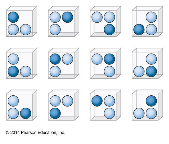
• Here are 12 distinct microstates
• All have the same properties
• Let the particle exert a pressure of p0 on the walls next to it
• Half the top walls have two particles next to it and half have one
• \(\expect{p_{top}} = 1.5p_0\)

The Microcanonical Ensemble

• Approaching a problem, we must decide which parameters are allowed to vary
• More flexible is more realistic but more difficult to solve
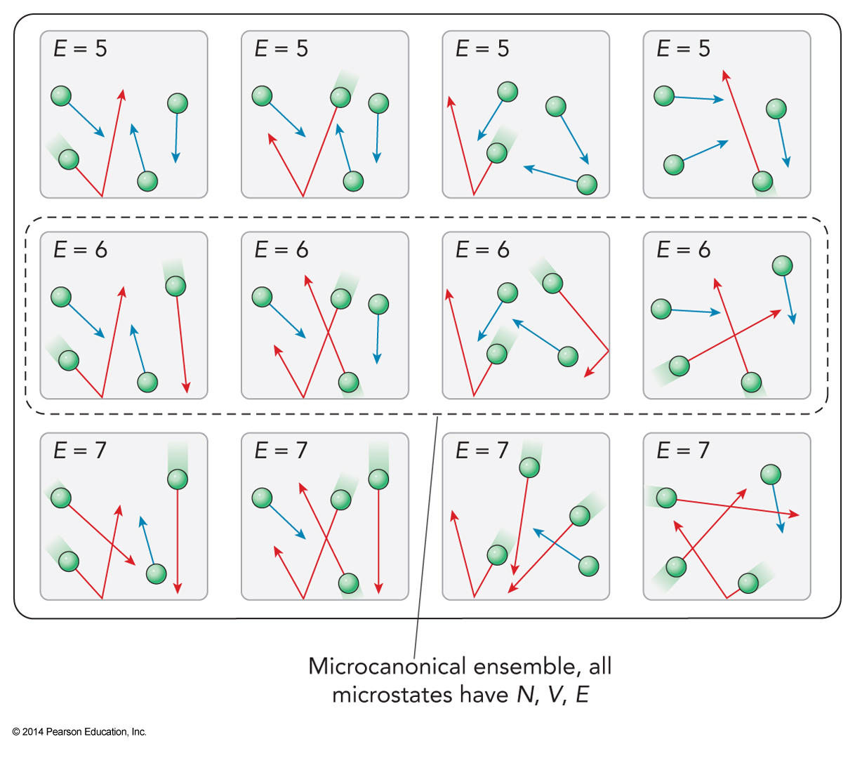
• If we fix all the extensive variables, \(E\), \(V\), and \(N\) we have our first ensemble – the microcanonical ensemble

Properties of Microcanonical Ensemble

• If we fix all extensive variables then intensive variables that are ratios of extensive variables must also be fixed
  • Density, \(\rho=\frac{N}{V}\)
• What can change?
  • Microscopic properties that we’re not bothering to measure
  • Some intensive properties (such as pressure) that are not ratios of extensive variables

Advantages of Microcanonical Ensemble

• Energy and mass are rigorously conserved
• There system must be completely isolated from the rest of the universe
• Constant volume means that no mechanical force pushes on the surroundings
• Isolation greatly simplifies the system

Entropy

Boltzmann Entropy

• The Boltzmann entropy is given by $$ S\equiv k_\mathrm{B}\ln \Omega $$
  • Boltzmann constant is \(k_\mathrm{B}=1.381\times 10^{-23}\,\mathrm{J}\,\mathrm{K}^{-1}\)
• This provides a different definition of the relation between heat and temperature
• This will be our rigorous definition of entropy since it works under and circumstances
• The entropy counts the total number of distinct microstates of the system

Entropy and Microstates

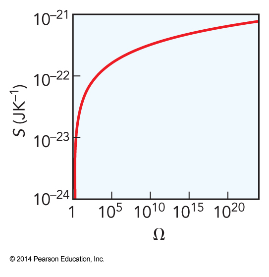
\(\Omega\) versus \(g\)

• For a microcanonical ensemble
  • \(\Omega\) is the total number of microstates that have the same energy
  • Under these conditions \(\Omega\) is the same as \(g\)
• \(\Omega\) is the total number of microstates in an ensemble
• \(g\) is the degeneracy of quantum states in some particular individual particle

Size of \(\Omega\)

• \(\Omega\) is enormous
• However, \(\Omega\) is always finite
  • The number of arrangements of system is countable
• In a classical system, \(\Omega\) would be infinite due to the continuous nature of classical mechanics
• Quantization makes \(\Omega\) finite

Two Non-Interacting Subsystems

• The degeneracy is the product of degeneracies
• The entropy is the sum of the entropies $$ \begin{align} \Omega_{\chem{A+B}} &= \Omega_\chem{A}\Omega_\chem{B} \\ \ln \Omega_{\chem{A+B}} &= \ln \left(\Omega_\chem{A}\Omega_\chem{B}\right) = \ln \Omega_\chem{A}+\ln \Omega_\chem{B} \\ S_\chem{A+B} &= S_\chem{A}+S_\chem{B} \end{align} $$

Gibbs Definition of Entropy

• Gibbs developed a general equation for estimating the entropy in any ensemble using probability rather than \(\Omega\)
• Derivation:
  • The total number of ways of arranging the labels on \(N\) molecules is \(N!\)
  • There are a total of \(N_i!\) ways of rearranging the labels

Example of Calculating \(\Omega\)

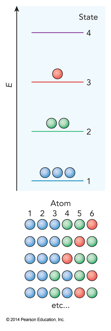
The Ensemble Size

• These definitions mean that we get $$ \Omega=\frac{N!}{N_1!N_2!N_3!\dots N_k!} = \frac{N!}{\prod_{i=1}^kN_i!} $$
• Example: 6 particles with 4 possible states with 3 in state 1, 2 in state 2, 1 in state 3 and 0 in state 4 $$ \Omega = \frac{6!}{(3!)(2!)(1!)(0!)}=60 $$
• Using this definition of the size of the ensemble we find $$ \begin{align} S &= k_\mathrm{B} \ln \Omega = k_\mathrm{B} \ln \left( \frac{N!}{\prod_{i=1}^kN_i!} \right) \\ &= k_\mathrm{B} \left[ \ln N! - \ln \prod_{i=1}^k N_i! \right] \end{align} $$

Using Stirling's Approximation

$$ S = k_\mathrm{B} \left[ \ln N! - \ln \prod_{i=1}^k N_i! \right] $$

• Now we can use Stirling’s approximation: \( \ln N! \approx N\ln N\) to yield $$ \begin{align} S &= k_\mathrm{B} \left[ N\ln N - N - \left( \sum_{i=1}^k N_i \ln N_i - \sum_{i=1}^k N_i \right) \right] \\ &= k_\mathrm{B} \left[ \sum_{i=1}^k N_i \ln N - N - \sum_{i=1}^k N_i \ln N_i +N \right] \\ &= k_\mathrm{B} \sum_{i=1}^k \left[ N_i \ln N - N_i \ln N_i \right] \\ &= k_\mathrm{B} \sum_{i=1}^k N_i \left[ \ln N - \ln N_i \right] \end{align} $$

Rewriting Entropy in Terms of Probability

$$ S = k_\mathrm{B} \sum_{i=1}^k N_i \left[ \ln N - \ln N_i \right] $$

• We can write this in terms of probabilities \(\mathcal{P}(i)=\frac{N_i}{N}\) $$ \begin{align} S &= Nk_\mathrm{B} \sum_{i=1}^k \frac{N_i}{N} \ln \frac{N}{N_i} \\ &= Nk_\mathrm{B} \sum_{i=1}^k \mathcal{P}(i) \ln \frac{1}{\mathcal{P}(i)} \\ &= -Nk_\mathrm{B} \sum_{i=1}^k \mathcal{P}(i) \ln \mathcal{P}(i) \end{align} $$

Temperature and the Partition Function

The Ideal Gas

• A collection of particles
• Don’t interact with each other at all
• Elastically bounce off walls
• We want to use statistical mechanics to find the pressure exerted by an ideal gas on the walls of the container as a function of the macroscopic variables

System and Reservoir

• The box has:
  • Fixed volume, \(V\)
  • Fixed number of molecules, \(N\)
• Energy will no longer be held constant
• Reservoir strongly interacts with system

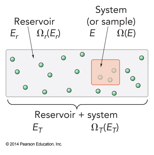
The Reservoir

• The reservoir has:
  • \(E_r \gg E\)
  • \(E+E_r = E_T \gg E\)
• \(\Omega_r\left(E_r\right) \gg \Omega\left(E\right)\)
• The ensemble size of the universe is $$ \Omega_T\left(E_T\right) = \sum_E \Omega\left(E\right) \Omega_r \left(E_r\right) $$

\(\mathcal{P}(i)\) and Number of Microstates

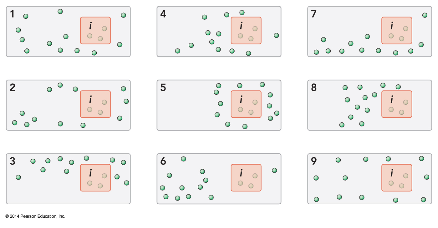
• Choose a single microstate, \(i\), with energy \(E_i\)
• If there are 9 distinct microstates with energy the reservoir must be changing
• Thus we can determine the system number from the reservoir number (\(E_r=E_T-E\))
• The probability of the system being in state \(i\) is $$ \mathcal{P}(i)=\frac{\Omega_r\left(E_r\right)}{\Omega_T\left(E_T\right)} $$

Ensemble Average

A Problem

• The problem is we don’t want to have to measure the reservoir instead of the system
• First we will rewrite this in terms of entropy (Taylor series expansion) $$ S_r \left( E_r \right) = S_r \left( E_T-E_i \right) = S_r \left( E_T \right) - \left. \left( \frac{\partial S_r}{\partial E_r} \right)_{V,N} \right|_{E_T} E_i + \cdots $$
• For a fixed total energy we know that \(dE_T = d\left(E_T-E\right)=-dE\)
• We also know that \(\Omega_T\left(E_T\right)=\Omega_r\left(E_r\right)\Omega\left(E\right)\)

Continuing to Solve the Problem

• We also know that $$ \begin{align} dS_r &= k_\mathrm{B} d \ln \Omega_r \left(E_r\right) = k_\mathrm{B} d\left[ \ln \left( \frac{\Omega_T\left(E_T\right)}{\Omega\left(E\right)} \right) \right] \\ &= k_\mathrm{B} d \left[ \ln \Omega_T \left(E_T\right) - \ln \Omega\left(E\right) \right] = -k_\mathrm{B} d\ln \Omega\left(E\right) \\ &= -dS \end{align} $$
• Combining these equations we find that $$ \left. \left( \frac{\partial S_r\left(E_r\right)}{\partial E_r} \right) \right|_{E_T} = \left. \left( \frac{\partial S(E)}{\partial E} \right) \right|_{E_T} $$

Rewriting the Entropy Equation

• Using these previous equation we find $$ S_r\left(E_r\right) = S_r\left(E_T-E_i\right) = S_r\left(E_T\right) - \left. \left( \frac{\partial S(E)}{\partial E} \right) \right|_{E_T} E_i $$
• This introduces temperature $$ T \equiv \left( \frac{\partial E}{\partial S} \right)_{V,N} $$
• Using temperature in the entropy equation $$ S_r\left(E_r\right) = S_r\left(E_T-E_i\right)=S_r\left(E_T\right)-\frac{E_i}{T} $$

Solving the Issues

• We can now go back to \(\Omega\) $$ k_\mathrm{B} \ln \left[ \Omega_r\left(E_r\right) \right] = k_\mathrm{B} \ln \left[ \Omega_r\left(E_T\right) \right] -\frac{E_i}{T} $$
• Solving for the number of reservoir states we get $$ \Omega_r\left(E_r\right)=\Omega_r\left(E_T\right)e^{-\bfrac{E_i}{k_\mathrm{B}T}} $$

Temperature

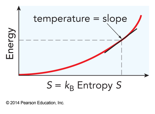
A New Ensemble

• In typical experiments, the energy is not fixed
  • The system and the surroundings/reservoir can exchange energy
• If the reservoir is big enough, its properties are constant, so we fix \(T\)
• So a canonical ensemble has \(T\), \(V\), and \(N\) fixed and \(E\) as a variable

More Equations, Now Within the Canonical Ensemble

• Combining some previous equations $$ \mathcal{P}(i)=\frac{\Omega_r\left(E_T\right)}{\Omega_T\left(E_T\right)} e^{-\bfrac{E_i}{k_\mathrm{B}T}} $$
• The \(\Omega\) are constants
• We can eliminate them by requiring that the probability be normalized $$ \sum_{i=1}^\infty \mathrm{P}(i) = \frac{\Omega_r\left(E_T\right)}{\Omega_T\left(E_T\right)} \sum_{i=1}^\infty e^{-\bfrac{E_i}{k_\mathrm{B}T}} = 1 $$

Solving the Equation

$$ \sum_{i=1}^\infty \mathrm{P}(i) = \frac{\Omega_r\left(E_T\right)}{\Omega_T\left(E_T\right)} \sum_{i=1}^\infty e^{-\bfrac{E_i}{k_\mathrm{B}T}} = 1 $$

• Solving for our fraction $$ \frac{\Omega_r\left(E_T\right)}{\Omega_T\left(E_T\right)} = \frac{1}{\sum_{i=1}^\infty e^{-\bfrac{E_i}{k_\mathrm{B}T}}} = \frac{1}{Q(T)} $$
• We have made a definition of the partition function

Canonical Partition Function and Distribution

• So, the canonical partition function is $$ Q(T)=\sum_{i=1}^\infty e^{-\bfrac{E_i}{k_\mathrm{B}T}} $$
• The canonical distribution can be written as $$ \mathcal{P}(i) = \frac{e^{-\bfrac{E_i}{k_\mathrm{B}T}}}{Q(T)} $$

Meaning

$$ \mathcal{P}(i) = \frac{e^{-\bfrac{E_i}{k_\mathrm{B}T}}}{Q(T)} $$

• We see the importance of \(T\)
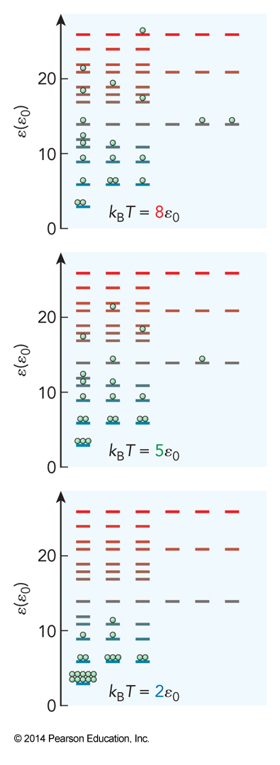
• The likelihood of getting the system into a particular state \(i\) drops exponentially with respect to the ratio of the microstate energy \(E_i\) to the thermal energy \(k_\mathrm{B}T\)
• The temperature establishes how likely the system is to be found at any particular energy.

Distribution in a 3D Box

Finding Another Likelihood

• Let’s find the likelihood of finding the system t any particular energy E $$ \mathcal{P}(E)=\Omega(E)\mathcal{P}(i) = \frac{\Omega(E) e^{-\bfrac{E_i}{k_\mathrm{B}T}}}{Q(T)} $$
• In all these equation the beauty of the canonical ensemble is that is allows us to ignore how \(\Omega\) depends on \(V\) and \(N\)

Assertion

• The probability extends to the probability of a particle within our system having some particular energy \(\varepsilon\)
• Say we have a particular quantum state \(i\) and degeneracy \(g\) $$ \begin{align} \mathcal{P}(\varepsilon) &= \frac{g(E) e^{-\bfrac{\varepsilon}{k_\mathrm{B}T}}}{q(T)} \\ q(T) &= \sum_{\varepsilon=0}^\infty g(E) e^{-\bfrac{\varepsilon}{k_\mathrm{B}T}} \end{align} $$

Rotational Partition Functions

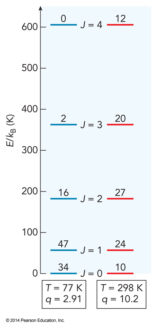
Check of Zero Energy

• If we measure all energy relative to \(E_0\) then $$ \begin{align} \mathcal{P}(E) &= \frac{ge^{-\bfrac{\left(E-E_0\right)}{k_\mathrm{B}T}}}{\sum_E ge^{-\bfrac{\left(E-E_0\right)}{k_\mathrm{B}T}}} \\ &= \left( \frac{ge^{-\bfrac{E}{k_\mathrm{B}T}}}{\sum_E ge^{-\bfrac{E}{k_\mathrm{B}T}}} \right) \left( \frac{e^{-\bfrac{E_0}{k_\mathrm{B}T}}}{e^{-\bfrac{E_0}{k_\mathrm{B}T}}} \right) = \frac{ge^{-\bfrac{E}{k_\mathrm{B}T}}}{\sum_E ge^{-\bfrac{E}{k_\mathrm{B}T}}} \end{align} $$

Example 2.1

At 298 K, calculate the ratio of the number of \(\chem{NH_3}\) molecules in the excited state to the number in the ground state, where the excited state is (a) the \(0^-\) state of the inversion, which lies \(0.79\,\mathrm{cm}^{-1}\) above the \(0^+\) ground state; and (b) the \(1^+\) state, which lies \(932.43\,\mathrm{cm}^{-1}\) above the \(0^+\). (The wavenumber unit, \(\mathrm{cm}^{-1}\), is conventionally used by spectroscopist as an energy unit, based on the relation between the transition energy in the experiment and the reciprocal wavelength of the photon that induces the transition: \(E_{photon}=\frac{hc}{\lambda}\). Because the energy is inversely proportional to the wavelength, energy is given in units of \(\frac{1}{\text{distance}}\).)

Example 2.2

At a temperature of 1000 K, how many vibrational states of \(\chem{H_2}\) are populated by at least 1% of the molecules, given the vibrational constant \(\omega_e=4395\,\mathrm{cm}^{-1}\) and the vibrational energy (relative to the ground state)of approximately \(E_{vib}=\omega_e\nu\)?

Example 2.3

You discover a molecular system having the energy levels and degeneracies $$ \varepsilon = c\left(n-1\right)^6;\;g=n;\;\text{for }n=1,2,3,\dots\text{ and }k_\mathrm{B}T=400c $$ Evaluate the partition function and calculate \(\mathcal{P}(\varepsilon)\) for each of the four lowest energy levels.

The Ideal Gas Law

The Original Problem - Pressure of an Ideal Gas

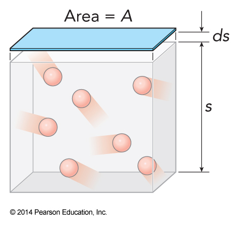
Moving A Wall

• We momentarily free one wall
• It reduces its forces therefore its pressure on the gas, \(P_{min}\)
• The gas pushes the wall out infinitesimally, \(ds\)

• The energy spent moving the wall is \(dE=-F\,dS = -P_{min} A\,dS = -P_{min} \,dV\)

The Pressure Equation

• If we hold \(N\) and \(S\) constant then $$ P_{min} = -\left( \frac{\partial E}{\partial V}\right)_{S,N} $$
• Mostly we will deal with the case where \(P\cong P_{min}\) $$ \text{if}\,P=P_{min}:P=-\left(\frac{\partial E}{\partial V}\right)_{S,N} $$

Cyclic Rule for Partial Derivatives

• The cyclic rule for partial derivatives is $$ \left( \frac{\partial X}{\partial Y}\right)_Z = -\left( \frac{\partial X}{\partial Z}\right)_Y\left(\frac{\partial Z}{\partial Y}\right)_X $$
• This allows us to write $$ P=-\left(\frac{\partial E}{\partial V}\right)_{S,N} = \left(\frac{\partial E}{\partial S}\right)_{V,N} \left(\frac{\partial S}{\partial V}\right)_{E,N} $$
• Another equation for temperature $$ T=\left(\frac{\partial E}{\partial S}\right)_{V,N} $$

Determining Entropy Change with Volume

• Let the translational states of the gas correspond to all the possible ways the gas particles can be arranged inside our box, regardless of what energy the gas has
• The box has a volume \(V\)
• Break up the volume into units \(V_0\), each able to hold a single particle
• We have \(M\) number of units so \(V=MV_0\)

More On Our Gas

• The particles are indistinguishable
• This reduces the number of distinct states
• If we had two particles the number of distinct states would be \(\bfrac{M\left(M-1\right)}{2}\)
• Extending this to \(N\) particles $$ \frac{M(M-1)(M-2)\dots (M-N)}{N!} $$
• For a gas \(M \gg N\)

Even More on Our Gas

• Introduce a constant \(A\) to absorb any other parameter’s effects, such as energy $$ \Omega = \lim_{M\gg N} A\frac{1}{N!} M(M-1)(M_2)\dots (M_N)=A\frac{1}{N!}M^N $$
• Because \(V=MV_0\) $$ \Omega\frac{1}{N!}\left(\frac{V}{V_0}\right)^N = A\frac{1}{V_0^NN!} V^N $$

The Entropy

• Ignoring everything but the volume dependence $$ \begin{align} S &= k_\mathrm{B} \ln \Omega = k_\mathrm{B} \ln \left[ \text{constant}\cdot V^N \right] \\ &= k_\mathrm{B} \left[ \ln \text{constant} + N\ln V\right] \end{align} $$
• This gives $$ \left(\frac{\partial S}{\partial V}\right)_{E,N} = k_\mathrm{B}N\left(\frac{\partial \ln V}{\partial V}\right)_{E,N} = k_\mathrm{B} \frac{N}{V} $$
• So $$ P=\left(\frac{\partial E}{\partial S}\right)_{V,N}\left(\frac{\partial S}{\partial V}\right)_{E,N} = \frac{k_\mathrm{B}TN}{V} $$

So What?

• Remember that \(k_\mathrm{B}\mathcal{N}_\mathrm{A}=R\)
• So $$ \begin{align} P &= \frac{k_\mathrm{B}TN}{V} = \frac{\frac{R}{\mathcal{N}_\mathrm{A}}TN}{V} = \frac{RT\frac{N}{\mathcal{N}_\mathrm{A}}}{V} = \frac{RTn}{V} \\ PV &= nRT \end{align} $$
• We managed to derive the classical ideal gas law equation from statistical mechanics using a canonical ensemble!