Mixtures and Solutions
Shaun Williams, PhD
Thermodynamics of Mixing
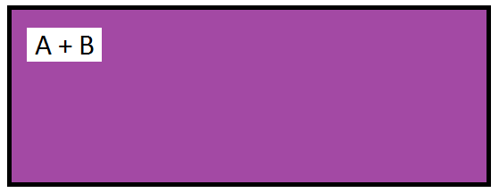
- Consider a sample of two gases filling two chambers in a single container
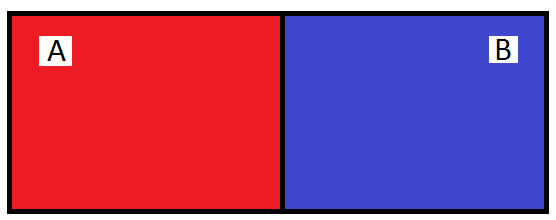
- After we remove the barrier and they mix isothermally, the partial pressures of the two gases will drop by a factor of 2 while the volume will double
Enthalpy of Mixing
- Assuming an ideal gas, let's look at the change in enthalpy of mixing
- The total enthalpy of mixing is \( \Delta H_{mix} = \Delta H_A + \Delta H_B \)
- Since the enthalpy change is for an isothermal expansion we know that \( \Delta H_{mix}=0 \)
- This will be true for ideal mixtures
Entropy of Mixing
- The entropy change due to the isothermal mixing is again the sum of the isothermal expansions of the two gases
- Entropy changes for isothermal expansions are easy to calculate for ideal gases \[ \Delta S = nR \ln \left( \frac{V_2}{V_1} \right) \]
- If we use \(V_A\) and \(V_B\) for the initial volumes of gases A and B then the total volume is \(V_A+V_B\) so \[ \Delta S_{mix} = n_A R \ln \left(\frac{V_A+V_B}{V_A}\right) + n_B R \ln \left(\frac{V_A+V_B}{V_B}\right) \]
Final Expression of the Entropy of Mixing
\( \Delta S_{mix} = n_A R \ln \left(\frac{V_A+V_B}{V_A}\right) + n_B R \ln \left(\frac{V_A+V_B}{V_B}\right) \)
- Note that (\(\chi_A\) is the mole fraction of A) \[ \frac{V_{tot}}{V_A} = \frac{V_A+V_B}{V_A} = \frac{1}{\chi_A} = \frac{n_A+n_B}{n_A} = \frac{n_{tot}}{n_A} \]
- Plugging in our mole fractions \[ \Delta S_{mix} = n_{tot}\chi_A R \ln \left(\frac{1}{\chi_A}\right) + n_{tot}\chi_B R \ln \left(\frac{1}{\chi_B}\right) \] \[ \Delta S_{mix} = n_{tot} R \left[ -\chi_A \ln \left(\chi_A\right) - \chi_B \ln \left( \chi_B \right) \right] \]
Analysis of the Entropy of Mixing
\[ \Delta S_{mix} = n_{tot} R \left[ -\chi_A \ln \left(\chi_A\right) - \chi_B \ln \left( \chi_B \right) \right] \]
- It is important to note that mole fractions (\(\chi\)) are always between 0 and 1 (0% - 100%).
- Because \(0\le\chi\le 1\) then \(\ln \chi \lt 0\) and \(-\ln \chi \gt 0\).
- The entropy change for a system undergoing isothermal mixing is always positive.
Free Energy of Mixing
- For isothermal mixing and constant total pressure \[ \Delta G_{mix} = \Delta H_{mix} - T \Delta S_{mix} \]
- Remember that for isothermal, \( \Delta H=0\) therefore \[ \Delta G_{mix} = n_{tot} RT \left[ \chi_A \ln \left(\chi_A\right) + \chi_B \ln \left( \chi_B \right) \right] \]
Plot of Mixing Energetics
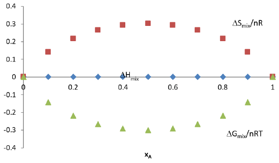
- Here we see that mixing at any level always has \(\Delta G_{mix}\lt 0\) and therefore it is always spontaneous - Mixing is always a spontaneous process for an ideal solution
Partial Molar Volume
- The partial molar volume of compound A in a mixture of A and B can be defined as \[ V_A = \left(\frac{\partial V}{\partial n_A}\right)_{P,T,n_B} \]
- So the total differential of \(V\) is \[ dV = \left(\frac{\partial V}{\partial n_A}\right)_{P,T,n_B} dn_A + \left(\frac{\partial V}{\partial n_B}\right)_{P,T,n_A} dn_B = V_A dn_A + V_B dn_B \]
An Integrated Version
\[ dV = V_A dn_A + V_B dn_B \]
- We can integrate this equation \[ \begin{eqnarray} V &=& \int_0^{n_A} V_A dn_A + \int_0^{n_B} V_B dn_B \\ &=& V_A n_A + V_B n_B \end{eqnarray} \]
- Overall, if \(\xi_i\) is the partial molar property \(X\) for component \(i\) of a mixture then the total property \(X\) for the mixture is \[ X=\sum_i \xi_i n_i \]
Chemical Potential
- Just like with the partial molar volume, we can define the partial molar Gibbs function \[ \mu_i = \left(\frac{\partial G}{\partial n_i}\right)_{P,T,n_{j\ne i}} \]
- \(\mu_i\) is called the chemical potential
- The chemical potential tells ho the Gibbs function will change as the composition of the mixture changes
- The chemical potential will point to the direction the system can move in order to reduce the total Gibbs function
A New Expression for the Total Gibbs Function
- The total change in the Gibbs function (\(dG\)) can be calculated from \[ dG = \left(\frac{\partial G}{\partial P}\right)_{T,n_i} dP + \left(\frac{\partial G}{\partial T}\right)_{P,n_i} dT + \sum_i \left(\frac{\partial G}{\partial n_i}\right)_{T,n_{j\ne i}} dn_i\]
- We could also substitute the chemical potentials and evaluating the pressure and temperature derviates as we have done in the past \[ dG = V\, dP-S\, dT+\sum_i \mu_i\, dn_i \]
Various Forms of the Chemical Potentials
| Thermodynamic Function | Chemical Potential Definition |
|---|---|
| \(dU=TdS-PdV+\sum_i \mu_idn_i\) | \(\mu_i=\left(\frac{\partial U}{\partial n_i}\right)_{S,V,n_{j\ne i}}\) |
| \(dH=TdS-VdP+\sum_i \mu_idn_i\) | \(\mu_i=\left(\frac{\partial H}{\partial n_i}\right)_{S,P,n_{j\ne i}}\) |
| \(dA=-PdV-SdT+\sum_i \mu_idn_i\) | \(\mu_i=\left(\frac{\partial A}{\partial n_i}\right)_{V,T,n_{j\ne i}}\) |
| \(dG=VdP-SdT+\sum_i \mu_idn_i\) | \(\mu_i=\left(\frac{\partial G}{\partial n_i}\right)_{P,T,n_{j\ne i}}\) |
Let's Look Farther into Chemical Potential
- If \(\mu_i=\left(\frac{\partial G}{\partial n_i}\right)_{P,T,n_{j\ne i}}\) and then \(dG=VdP-SdT+\sum_i \mu_idn_i\) then \[ d\mu = VdP-SdT \]
- From this we see that \[ \left(\frac{\partial \mu}{\partial P}\right)_T=V \xrightarrow{\Delta T=0} \int_{\mu^\circ}^{\mu}d\mu = \int_{P^\circ}^P VdP\]
Defining Chemical Potentials
- For substances for which the molar volume is mostly independent of pressure at constant temperature (small \(\kappa_T\) \[ \begin{eqnarray} \int_{\mu^\circ}^{\mu}d\mu &=& V \int_{P^\circ}^P dP \\ \mu-\mu^\circ &=& V\left(P-P^\circ\right) \\ \mu &=& \mu^\circ + V\left(P-P^\circ\right) \end{eqnarray} \] where \(P^\circ\) is a reference pressure and \(\mu^\circ\) is the chemical potential at the standard pressure
What About for Highly Compressible Materials?
- If we have a highly compressible ideal gas we can use \(V=\frac{RT}{P}\) so that at constant temperature \[ \int_{\mu^\circ}^\mu d\mu = RT\int_{P^\circ}^P \frac{dP}{P} \] or \[ \mu = \mu^\circ + RT \ln \left(\frac{P}{P^\circ}\right) \]
The Gibbs-Duhem Equation
- For a system at equilibrium, the Gibbs-Duhem equation must hold \[ \sum_i n_i\,d\mu_i =0 \]
- Since \(\mu_i\) is the partial Gibbs function for component \(i\) \[ G_{tot}=\sum_i n_i\mu_i \] \[ dG_{tot}=\sum_i n_i\,d\mu_i + \sum_i \mu_i\,dn_i \]
Another Expression for \(dG\)
- From before we know that \[ dG=VdP-SdT+\sum_i\mu_idn_i \]
- Setting this equal to the expression for \(dG_{tot}\)\(\require{cancel}\) \[ \sum_i n_id\mu_i + \cancel{\sum_i \mu_i dn_i} = VdP-SdT+\cancel{\sum_i \mu_idn_i} \] \[ \sum_i n_id\mu_i = VdP-SdT \]
Finishing the Derivation of the Gibbs-Duhem Equation
\[ \sum_i n_id\mu_i = VdP-SdT \]
- If the system is at constant temperature and pressure then \(dP=0\) and \(dT=0\) therefore \(VdP-SdT=0\) and therefore \[ \sum_i n_i d\mu_i=0 \]
A Binary System
- For a binary system of components A and B at equilibrium \[ \sum_i n_id\mu_i = n_Ad\mu_A + n_B d\mu_B =0 \] \[ d\mu_B = -\frac{n_A}{n_B}d\mu_A \]
Non-Ideality in Gases - Fugacity
- So far, we only have an ideal gas equation for the chemical potential \[ \mu = \mu^\circ + RT \ln \left(\frac{P}{P^\circ}\right) \]
- We often want to deal with real gases that deviate from ideal behavior
- To do deal with non-ideality, we need a "fudge" factor called fugacity, \(f\)
Fugacity
- Fugacity is related to pressure but contains all the deviations from ideality \[ \mu = \mu^\circ + RT\ln \left(\frac{f}{f^\circ}\right) \]
- Let's look at how \(f\) is related to \(P\)
- Consider the change in the chemical potential for a one component system \[ d\mu=VdP-SdT \therefore \left(\frac{\partial \mu}{\partial P}\right)_T=V \]
How Fugacity and Pressure are Related
- Let's plug in the actual chemical potential into the derivative. \[ \left(\frac{\partial \mu}{\partial P}\right)_T = \left\{ \frac{\partial}{\partial P} \left[ \mu^\circ + RT\ln \left(\frac{f}{f^\circ}\right) \right] \right\} \] \[ \left(\frac{\partial \mu}{\partial P}\right)_T = RT\left[ \frac{\partial \ln(f)}{\partial P} \right]_T \stackrel{\text{from before}}{=} V \]
- Multiplying by \(\frac{P}{RT}\) \[ P\left[ \frac{\partial \ln(f)}{\partial P} \right]_T = \frac{PV}{RT} = Z \] where \(Z\) is the compression factor
Fugacity Coefficient, \(\gamma\)
- Let's derive the fugacity coefficient, \(\gamma\) \[ f=\gamma P \]
- Taking the natural log of both sides \[ \ln f = \ln(\gamma P) = \ln \gamma + \ln P \] \[ \ln \gamma = \ln f - \ln P \]
Doing Some Calculus
- Plugging this into our previous equation and integrating \[ \int \left(\frac{\partial \ln \gamma}{\partial P}\right)_TdP = \int\left(\frac{\partial \ln f}{\partial P} - \frac{\partial \ln P}{\partial P}\right)_TdP \] \[ \int \left(\frac{\partial \ln \gamma}{\partial P}\right)_TdP = \int \left( \frac{Z}{P}-\frac{1}{P}\right)_TdP \] \[ \ln \gamma = \int_0^P \left(\frac{Z-1}{P}\right)_T dP \]
Colligative Properties
- Colligative properties describe how the properties of the solvent with change as solute (or solutes) are added.
- Solution - a homogeneous mixture
- Solvent - The component of a solution with the largest mole fraction
- Solute - Any component of a solution that is not the solvent
- While solutions can exist in solid, liquid, or gaseous phases, we will primarily deal with liquid-phase solutions.
Freezing Point Depression
- In general, a liquid will freeze when \[ \mu_{solid} \le \mu_{liquid} \]
- This means that the freezing point of a solvent will be affected by anything that changes the chemical potential of the solvent
- In a mixture, the chemical potential of component A is \[ \mu_A = \mu_A^\circ + RT\ln \chi_A \]
- Because \(\chi_A \le 1\), the chemical potential is always reduced by adding another component
Freezing Solvent
- A Solvent will freeze if \[ \mu_{A,solid}=\mu_{A,liquid} \]
- Because \(\mu_A = \mu_A^\circ + RT\ln \chi_A\) \[ \frac{\mu_A-\mu_A^\circ}{RT}=\ln \chi_A \]
- Let's look at the temperature dependence of the chemical potential \[ \left[ \frac{\partial}{\partial T} \left(\frac{\mu_A-\mu_A^\circ}{RT}\right) \right]_P = \left(\frac{\partial \ln \chi_A}{\partial T}\right)_P \]
The Temperature Dependence of \(\mu\)
\[ \left[ \frac{\partial}{\partial T} \left(\frac{\mu_A-\mu_A^\circ}{RT}\right) \right]_P = \left(\frac{\partial \ln \chi_A}{\partial T}\right)_P \] \[ -\frac{\mu_A-\mu_A^\circ}{RT^2} + \frac{1}{RT}\left[ \left(\frac{\partial \mu_A}{\partial T}\right)_P-\left(\frac{\partial \mu_A^\circ}{\partial T}\right)_P \right] = \left(\frac{\partial \ln \chi_A}{\partial T}\right)_P \] Because \(\mu=H-TS\) and \(\left(\frac{\partial \mu}{\partial T}\right)_P=-S\) \[ -\frac{H_A-TS_A-H_A^\circ+TS_A^\circ}{RT^2} + \frac{1}{RT}\left[ -S_A+S_A^\circ \right] = \left(\frac{\partial \ln \chi_A}{\partial T}\right)_P \]
Heat of Fusion
- In the case of the solvent freezing, \(H_A^\circ\) is the enthalpy of the pure solvent in solid form and \(H_A\) is the enthalpy of the solvent in the liquid solution
- This means that \[ H_A^\circ - H_A = \Delta H_{fus} \]
- So our equation becomes \[ \frac{\Delta H_{fus}}{RT^2} - \cancel{\frac{-S_A+S_A^\circ}{RT}}+\cancel{\frac{-S_A+S_A^\circ}{RT}} = \left(\frac{\partial \ln \chi_A}{\partial T}\right)_P \]
Integrating Our Equation
- Our equation reduced to \[ \frac{\Delta H_{fus}}{RT^2} = \left(\frac{\partial \ln \chi_A}{\partial T}\right)_P \]
- Seperating variable and integrating \[ \int_{T^\circ}^T \frac{\Delta H_{fus}}{RT^2}dT = \int d\,\ln \chi_A \] where \(T^\circ\) is the freezing point of the pure solvent and \(T\) is the temperature at which the solvent will begin to solidify in the solution
Doing the Integration
- After integration \[ -\frac{\Delta H_{fus}}{R}\left(\frac{1}{T}-\frac{1}{T^\circ}\right)=\ln \chi_A \]
- It is important to note that \( \frac{1}{T}-\frac{1}{T^\circ} = \frac{T^\circ-T}{TT^\circ} = \frac{\Delta T}{TT^\circ} \)
- For small deviations from the pure freezing point, \(TT^\circ \approx \left(T^\circ\right)^2\) \[ -\frac{\Delta H_{fus}}{R\left(T^\circ\right)^2}\Delta T = \ln \chi_A \]
Further Simplifications
- For dilute solutions, \(\chi_A\approx 1\) and therefore \(\ln \chi_A \approx 0\) so \[ \ln \chi_A \approx -(1-\chi_A) = -\chi_B \] where \(\chi_B\) is the mole fraction of the solute
- So we now have \[ -\frac{\Delta H_{fus}}{R\left(T^\circ\right)^2}\Delta T = \chi_B \] \[ \Delta T = \left(\frac{R\left(T^\circ\right)^2}{\Delta H_{fus}}\right)\chi_B \]
The Cryoscopic Constant, \(K_f\)
\[ \Delta T = \left(\frac{R\left(T^\circ\right)^2}{\Delta H_{fus}}\right)\chi_B \]
- The first term on the right-hand side is a constant \[ \frac{R\left(T^\circ\right)^2}{\Delta H_{fus}}=K_f \]
- This gives us an equation that you have seen in general chemistry \[ \Delta T = K_f \chi_B \]
Boiling Point Elevation
- The same derivation that we just finished can also be done for the boiling point with the same result.
- The increase in boiling point is \[ \Delta T=K_b \chi_B \] where \[ \frac{R\left(T^\circ\right)^2}{\Delta H_{vap}}=K_b \]
- \(K_b\) is called teh ebullioscopic constant
The Cryoscopic and Ebullioscopic Constants
- Both the cryoscopic and ebullioscopic constants are generally tabulated in terms of molality as the unit of solute concentration rather than mole fraction \[ \Delta T = K_f m \;\;\;\text{and}\;\;\; \Delta T=K_b m\]
A Selection of Cryoscopic and Ebullioscopic Constants
| Substance | \(K_f\, (^\circ C\,kg\,mol^{-1})\) | \(T_f^\circ\, (^\circ C)\) | \(K_b\, (^\circ C\,kg\,mol^{-1})\) | \(T_b^\circ\, (^\circ C)\) |
|---|---|---|---|---|
| Water | 1.86 | 0.0 | 0.51 | 100.0 |
| Benzene | 5.12 | 5.5 | 2.53 | 80.1 |
| Ethanol | 1.99 | -114.6 | 1.22 | 78.4 |
| \(\chem{CCl_4}\) | 29.8 | -22.3 | 5.02 | 76.8 |
Example 7.1
The boiling point of a solution of \(3.00\,g\) of an unknown compound in \(25.0\, g\) of \(\chem{CCl_4}\) raises the boiling point to \(81.5^\circ C\). What is the molar mass of the compound?
Vapor Pressure Lowering
- For the same reason as the lowering of freezing points nad raising of boiling points, the vapor pressure of volatile solvent will be decreased due to the introduction of a solute.
- In order to establish equilibrium between solvent in solution and vapor phase, the chemical potentials of the two phases must be equal \[ \mu_{vapor} = \mu_{solvent} \]
- If the solute is not volatile then the vapor will be pure solute so \[ \mu_{vap}^\circ + RT \ln \frac{P'}{P^\circ} = \mu_A^\circ +RT\ln \chi_A \] where \(P'\) is the vapor pressure of the solvent over the solution
Working on the Vapor Pressure
- Similarly for the pure solvent in equilibrium with its vapor \[ \mu_A^\circ = \mu_{vap}^\circ + RT \ln \frac{P_A}{P^\circ} \] where \(P^\circ\) is the standard pressure of 1 atm, and \(P_A\) is the vapor pressure of the pure solvent.
- Putting the last two equations together we find that \[ \cancel{\mu_{vap}^\circ} + RT \ln \frac{P'}{P^\circ} = \left( \cancel{\mu_{vap}^\circ} + RT \ln \frac{P_A}{P^\circ} \right) + RT\ln \chi_A \] \[ RT \ln \frac{P'}{P^\circ} = RT \ln \frac{P_A}{P^\circ} + RT\ln \chi_A \]
Raoult's Law
- Cancelling out the \(RT\) that is in every term and rearranging \[ \ln \frac{P'}{P^\circ} = \ln \frac{P_A}{P^\circ} + \ln \chi_A \] \[ \ln \frac{P'}{P^\circ} - \ln \frac{P_A}{P^\circ} = \ln \chi_A \Rightarrow \ln \frac{P'}{P^\circ}\frac{P^\circ}{P_A} = \ln \frac{P'}{P_A} = \ln \chi_A \] \[ \frac{P'}{P_A}=\chi_A \Rightarrow P'=\chi_AP_A \] This is Raoult's Law
Example 7.2
Consider a mixture of two volatile liquids A and B. The vapor pressure of pure A is \(150\,Torr\) at some temperature, and that of pure B is \(300\,Torr\) at the same temperature. What is the total vapor pressure above a mixtire of these compounds with the mole fraction of B of \(0.600\). What is the mole fraction of B in the vapor that is in equilibrium with the liquid mixture?
Osmotic Pressure
- Osmosis is a process by which a solvent can pass through a semi-permeable membrane from an area of low solute concentration to a region of high solute concentration
- The osmotic pressure is the pressure that when exeted on the region of high solute concentration will halt the process of osmosis
- The magnitude of the osmotic pressure can be understood by examining the chemical potential of a pure solvent and that of the solvent in a solution
Chemical Potentials in Osmosis
- The chemical potential of the solvent in the solution is given by \[ \mu_A = \mu_A^\circ +RT \ln \chi_A \]
- Since \(\chi_A\le 1\), the chemical potential of the solvent in a solution is always lower than in a pure solvent
- To prevent osmosis, something must be done to raise the chemical potential of the solvent in the solution
- This can be done by applying pressure (\(\pi\)) to the solution \[ \mu_A^\circ(P)=\mu_A(\chi_B,+\pi) \]
Solving for the Pressure
- We already know that the chemical potential of the solvent in the solution is reduced by an amount given by \[ \mu_A^\circ - \mu_A = RT\ln \chi_A \]
- The increase in chemical potential due to the application of excess pressure is given by \[ \mu(P+\pi)=\mu(P) + \int_P^{P+\pi} \left(\frac{\partial \mu}{\partial P}\right)_T dP \]
Simplifying The Expression
- We already know that \( \left(\frac{\partial \mu}{\partial P}\right)_T=V \)
- Combining some equations \[ -RT\ln \chi_A = \int_P^{P+\pi}V\,dP \]
- If the molar volume of the solvent is independent of pressure \[ -RT\ln \chi_A = V \left. P\right|_P^{P+\pi} = V\pi \]
Further Simplifications
- We have already seen that if \(\chi_A\approx 1\) then \[ \ln \chi_A \approx -(1-\chi_A)=-\chi_B \]
- So, for dilute solutions \[ \chi_B RT=V\pi \] \[ \pi = \frac{\chi_BRT}{V} \]
- For cases where \(n_B \ll n_A\) \[ \pi =\left[B\right]RT \]
Solubility
- The maximum solubility of a solute can be determined using the same methods used in the colligative properties.
- The chemical potential of the solute in a liquid solution \[ \mu_{B}(solution) = \mu_B^\circ(liquid)+RT\ln \chi_B \]
- If this chemical potential is lower than that of a pure solid solute, the solute will dissolve.
- The point of saturation is when the chemical potential of the solute in the solute is equal to that of the pure solid solute.
The Saturation Point
- Let's start by setting those chemical potentials equal \[ \mu_B^\circ(solid)=\mu_B^\circ(liquid)+RT\ln \chi_B \]
- We are interested in the mole fraction \[ \ln \chi_B = \frac{\mu_B^\circ(solid)-\mu_B^\circ(liquid)}{RT} \]
- The numerator is the molar Gibbs function of fusion, so \[ \ln \chi_B = \frac{-\Delta G_{fus}^\circ}{RT} \]
Getting to Enthalpy instead of Gibbs Function
- Remember the Gibbs-Helmholtz equation \[ \left(\frac{\partial \left(\frac{\Delta G}{T}\right)}{\partial T}\right)_P = \frac{\Delta H}{T^2} \]
- Let's take the derivative of out \(\ln \chi_B\) equation with respect to T at constant P \[ \left(\frac{\partial \ln \chi_B}{\partial T}\right)_P = \frac{1}{R}\frac{\Delta H_{fus}}{T^2} \]
Let's Separate the Variables and Integrate
- Let's separate the variables and integrate \[ \int_0^{\ln \chi_B} d\,\ln \chi_B = \frac{1}{R} \int_{T_f}^T \frac{\Delta H_{fus}\,dT}{T^2} \] \[ \ln \chi_B = \frac{\Delta H_{fus}}{R} \left(\frac{1}{T_f}-\frac{1}{T} \right) \]
Non-Ideality in Solutions - Activity
- So far we have dealt primarily ideal solutions
- Real solutions deviate rom ideal bahavior
- In the case of gases we used fugacity to account for ideality
- In the case of real solutes we use activity
- The activity of a solute is related to its concentration by \[ a_B = \gamma \frac{m_B}{m^\circ} \]
Activity
-
\[ a_B=\gamma \frac{m_B}{m^\circ} \]
- \(\gamma\) is the activity coefficient
- \(m_B\) is the molality of the solute
- \(m^\circ\) is unit molality
- We can add activity to our chemical potential \[ \mu_B=\mu_B^\circ + RT \ln a_B \]
- The measurements of the activity coefficients depend on temperature, pressure, and concentration
Activity Coefficients for Ionic Solutes
- For an ionic substance that dissociates when dissolved \[ \chem{MX(s)\rightarrow M^+(aq)+X^-(aq)} \] the chemical potential of the cation is \(\mu_+\) and that of the anion is \(\mu_-\)
- The total molar Gibbs function of the solute \[ G = \mu_+ + \mu_- \] where \[ \mu = \mu^* + RT\ln a \] where \(\mu^*\) is the chemical potential of an ideal solution
Gibbs Function of Solution
- Plugging the chemical activity into the Gibbs function \[ G = \mu_+^* + RT \ln a_+ + \mu_-^* + RT\ln a_- \]
- Using the molar definition of the activity coefficient \(a_i=\gamma_i m_i\) \[ G = \mu_+^* + RT \ln \gamma_+m_+ + \mu_-^* + RT\ln \gamma_-m_- \] \[ G = \mu_+^* + \mu_-^* + RT \ln \gamma_+m_+ + RT\ln \gamma_-m_- \] \[ G = \mu_+^* + \mu_-^* + RT \ln \gamma_+m_+ \gamma_-m_- \] \[ G = \mu_+^* + \mu_-^* + RT \ln m_+m_- + RT\ln \gamma_+\gamma_- \]
Mean Activity Coefficient
- It is impossile to deconvolve the term into specfic contributions of the two ions
- We use the geometric average to define the mean activity coefficient, \(\gamma_\pm = \sqrt{\gamma_+\gamma_-} \)
- For a substance the dissociates according to \[ \chem{M_xX_y(s)\rightarrow xM^{y+}(aq)+yX^{x-}(aq)} \] the expression for the mean activity coefficient if given by \[ \gamma_\pm = \left(\gamma_+^x\gamma_-^y\right)^{\bfrac{1}{x+y}} \]
Debeye-Hückel Law
- In 1923, Debeye and Hückel suggested a means of calculating the mean activity coefficients from experimental data \[ \log_{10}\gamma_\pm = \frac{1.824\times 10^6}{\left(\epsilon T\right)^\bfrac{3}{2}}\left| z_++z_-\right|\sqrt{I} \] where \(\epsilon\) is the dielectric constant of the solvent, \(T\) is the temperature in K, \(z_+\) and \(z_-\) are the charges on the ions, and \(I\) is the ionic strength
- \(I\) is given by \[ I=\frac{1}{2}\frac{m_+z_+^2+m_-z_-^2}{m^\circ} \]
/