Gases
Shaun Williams, PhD
The Empirical Gas Laws
Boyle's Law
- Robert Boyle (1627-1691) showed that for a fixed sample of gas at a constant temperature, pressure and volume are inversely proportional \[ P \propto \frac{1}{V} \] \[ PV = \text{constant} \] \[ P_1V_1 = P_2V_2 \]
Charles' Law
- Charles' Law states that the volume of a fixed sample of gas at constant pressure is proportional to the temperature. \[ V \propto T \] \[ \frac{V}{T} = \text{constant} \] \[ \frac{V_1}{T_1} = \frac{V_2}{T_2} \]
Gay-Lussac's Law
- Gay-Lussac's law states that the pressure of a fixed sample of gas is proportonal to the temperature \[ P \propto T \] \[ \frac{P}{T}=\text{constant} \] \[ \frac{P_1}{T_1}=\frac{P_2}{T_2} \]
Combined Gas Law
- Boyle's, Charles', and Gay-Lussac's Laws can be combined into a single empirical formula \[ PV \propto T \] \[ \frac{PV}{T}=\text{constant} \] \[ \frac{P_1V_1}{T_1}=\frac{P_2V_2}{T_2} \]
Avogadro's Law
- Amedeo Avogadro (1776-1856) did extensive work with gases
- Avogadro found an important relationship regarding the number of moles of gas when the temperature and pressure are constant \[ n \propto V \] \[ \frac{n}{V}=\text{constant} \] \[ \frac{n_1}{V_1}=\frac{n_2}{V_2} \]
The Ideal Gas Law
- The ideal gas law combines the empirical gas laws into a single expression in terms of the universal gas constant, \(R\) \[ PV=nRT \]
| Value | Unit | Value | Unit | |
|---|---|---|---|---|
| 8.3144598 | \( \frac{J}{mol\, K} \) | 1.9872036 | \( \frac{cal}{mol\, K} \) | |
| 0.082057338 | \( \frac{L\, atm}{mol\, K} \) | 0.0019872036 | \( \frac{kcal}{mol\, K} \) | |
| 0.083144598 | \( \frac{L\, bar}{mol\, K} \) |
Note: \( R=N_Ak_B \) where \( k_B = 1.38064852\times 10^{-23}\, \bfrac{J}{K} \) and \( N_A= 6.022140857\times 10^{23}\,mol^{-1} \)
The Kinetic Molecular Theory of Gases
The kinetic molecular theory of gases has 5 postulates in its modern form
- Gas particles obey Newton’s laws of motion and travel in straight lines unless they collide with other particles or the walls of the container.
- Gas particles are very small compared to the averages of the distances between them.
- Molecular collisions are perfectly elastic so that kinetic energy is conserved.
- Gas particles so not interact with other particles except through collisions. There are no attractive or repulsive forces between particles.
- The average kinetic energy of the particles in a sample of gas is proportional to the temperature.
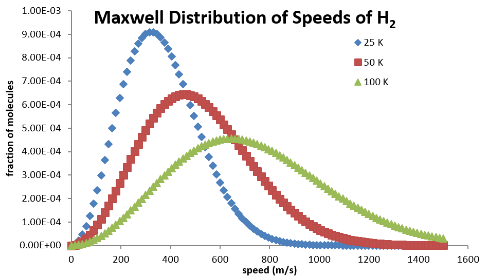
Maxwell Distribution of Speeds
- Based on the kinetic molecular theory of gases we can develop an expression of the fraction of gas particles with a specific speed \[ f(v) = 4\pi \sqrt{\left( \frac{m}{2\pi k_BT} \right)^3} v^2 \exp \left( -\frac{mv^2}{2k_BT} \right) \]
Calculating the Average Speed of a Gas
We can calculate the average molecular speed of a gas
\[ \begin{eqnarray} \left< v \right> &=& \int_{-\infty}^{\infty} v\,f(v)\,dv \\ &=& \int_{-\infty}^{\infty} v\, 4\pi \sqrt{\left( \frac{m}{2\pi k_BT} \right)^3} v^2 \exp \left( -\frac{mv^2}{2k_BT} \right)\,dv \\ &=& 4\pi \sqrt{\left( \frac{m}{2\pi k_BT} \right)^3} \int_{-\infty}^{\infty} v^3 \exp \left( -\frac{mv^2}{2k_BT} \right)\, dv \end{eqnarray} \]Solving the Integral
\[ \left< v \right> = 4\pi \sqrt{\left( \frac{m}{2\pi k_BT} \right)^3} \int_{-\infty}^{\infty} v^3 \exp \left( -\frac{mv^2}{2k_BT} \right)\, dv \]
We can find how to solve this integral in a table of integrals: \[ \int_0^\infty x^{2n+1} e^{-ax^2} \, dx = \frac{n!}{2a^{n+1}} \]
So \[ \begin{eqnarray} \left< v \right> &=& 4\pi \sqrt{\left( \frac{m}{2\pi k_BT} \right)^3} \left[ \frac{1}{2\left( \frac{m}{2k_BT} \right)^2} \right] \\ &=& \left(\frac{8k_BT}{\pi m}\right)^\bfrac{1}{2} \end{eqnarray} \]
Example 2.1
What is the average value of the squared speed according to the Maxwell distribution law?
Note: \( \int_0^\infty x^{2n}e^{-ax^2}\,dx=\frac{1\cdot 3\cdot 5\cdots (2n-1)}{2^{n+1}a^n}\sqrt{\frac{\pi}{a}} \)
Note 2: The root-mean-squared (RMS) speed of gas particle is the squareroot of the average value of \(v^2\) \[ v_{rms}=\sqrt{\left< v^2 \right>} \]
Kinetic Energy
Using expresson for \(v_{mp}\), \(v_{avg}\), and \(v_{rms}\) we can develop expression for the kinetic energy using \[ E_k=\frac{1}{2}mv^2 \]
| Property | Speed | Kinetic Energy |
|---|---|---|
| Most probable | \(\sqrt{\frac{2k_BT}{m}}\) | \(k_BT\) |
| Average | \(\sqrt{\frac{8k_BT}{\pi m}}\) | \(\frac{4k_BT}{\pi}\) |
| Root-mean-squared | \(\sqrt{\frac{3k_BT}{m}}\) | \(\frac{3}{2}k_BT\) |
Real Gases
The van der Waals Equation
- Johannes van der Waals (1837-1923) suggested an modified version of the ideal gas law to account for the deviations of real gases from ideality \[ \left( P+\frac{a}{V_m^2} \right)\left( V_m-b \right) = RT \]
| Gas | a (atm L2 mol-2) | b (L mol-1) |
|---|---|---|
| He | 0.0341 | 0.0238 |
| N2 | 1.352 | 0.0387 |
| CO2 | 3.610 | 0.0429 |
| C2H4 | 4.552 | 0.0305 |
Other Real Gas Laws
| Model | Equation of State |
|---|---|
| Ideal | \( P=\frac{RT}{V_m} \) |
| van der Waals | \( P=\frac{RT}{V_m-b}-\frac{a}{V_m^2} \) |
| Redlich-Kwong | \( P=\frac{RT}{V_m-b} - \frac{a}{\sqrt{T}V_m\left(V_m+b\right)} \) |
| Dieterici | \( P=\frac{RT}{V_m-b}\exp \left( \frac{-a}{V_mRT} \right) \) |
| Clausius | \( P=\frac{RT}{V_m-b}-\frac{a}{T\left(V_m+c\right)^2} \) |
| Virial Expansion | \( P=\frac{RT}{V_m}\left( 1+\frac{B(T)}{V_m}+\frac{C(T)}{V_m^2}\cdots \right) \) |
/