First Law of Thermodynamics
Shaun Williams, PhD
Work and Heat
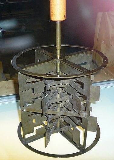
James P. Joule (1818-1889)
- Joule was one of the pioneers of modern thermodynamics.
- Among his experiments, Joule attempted to measure the effect of work on the temperature of water.
The First Law of Thermodynamics
The capacity of a system to do work is increased by heating the system or doing work on it.
- The first law translates to \[ \begin{eqnarray} \Delta U &=& q+w \\ dU &=& dq+dw \end{eqnarray} \]
Heat
- Heat is the flow of energy that, in the absence of other changes, will change the temperature of the system.
- Endothermic - heat flows into the system (\(q_{system}>0\))
- Exothermic - heat flows out of the system (\(q_{system}<0\))
- An infinitesimal amount of heat flowing can be related to the temperature change as \[ dq=C\,dT \] where \(C\) is the heat capacity.
Example 3.1
How much energy is needed to raise the temperature of \(5.0\, g\) of water from \(21.0^\circ C\) to \(25.0^\circ C\)?
Side Note: Partial Derivative
- The ideal gas law tells us that \[ P(V,n,T)=\frac{nRT}{V} \]
- How do we calculate the infinitesimal change in the pressure (\(dP\)) if all the variable can change?
- The infinitesimal change in any function can be calculated as \[ df = \sum_i \left( \frac{\partial f}{\partial x_i} \right)_{x_j\ne i} dx_i\]
Work
- Work can take various forms, some of which we have already spoken about
| Type of Work | Displacement | Resistance | \(dw=\) |
|---|---|---|---|
| Expansion | \( dV \) (volume) | \( -P_{ext} \) (pressure) | \( -P_{ext}\,dV \) |
| Electrical | \( dQ \) (charge) | \( -W \) (resistance) | \( -W\,dQ \) |
| Extension | \( dL \) (length) | \( T \) (tension) | \( T\,dL \) |
| Stretching | \( dA \) | \( s \) (surface tension) | \( s\,dA \) |
Example 3.2
What is the work done by \( 1.00\, mol\) of an ideal gas expanding from a volume of \( 22.4\, L \) to a volume of \( 44.8\, L \) against a constant external pressure of \( 0.500\, atm \)?
Reversible and Irreversible Pathways
Reversible Gas Expansions
- Imagine a gas in a cylinder (with a piston) where the pressure of the gas and the external pressure are the same.
- There is no spontaneous change of the gas towards seeking larger or smaller volume
- Since the internal pressure (\(P\)) and the external pressure (\(P_{ext}\)) are the same \[ dw=-P_{ext}\, dV = -P\, dV \]
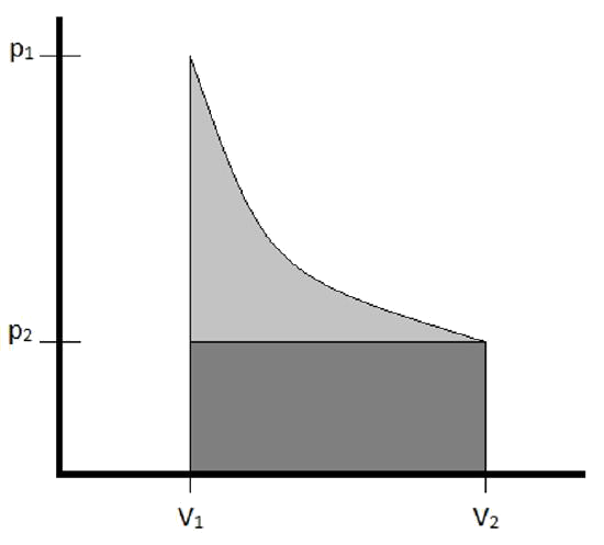
Solving Reversible Gas Expansion
\( dw = -P_{ext}\, dV = -P\, dV \)
\[ \begin{eqnarray} w &=& - \int P\,dV \\ &=& -\int \left(\frac{nRT}{V}\right) \\ &=& -nRT \int_{V_1}^{V_2} \frac{dV}{V} = -nRT \ln \left(\frac{V_2}{V_1}\right) \end{eqnarray} \]Example 3.3
What is the work done by \( 1.00\, mol \) of an ideal gas expanding reversibly from a volume of \( 22.4\, L \) to a volume of \( 44.8\, L \) at a constant temperature of \( 273\, K \)?
Note: Isothermal Processes of an Ideal Gas
- Isothermal means the process occurs at a constant temperature
- Ideal gases, due to its assumptions, can only store energy as kinetic energy
- Changing kinetic energy means changing temperature
- So, no change in temperature means no change in \( U \)
- \( \Delta U=0 \therefore q=-w \) for isothermal processes involving ideal gases
Constant Volume "Expansion" - Isochoric
- If a gas is constrained by sufficient force, it cannot change volume therefore \( dV=0 \)
- So, \[ dU=dq+dw=dq-P\,dV=dq \]
- Since, \( dq=C\, dT \) \[ dU = C\, dT \]
- This gives us an important definition for the constant volume heat capacity \[ C_V \equiv \left( \frac{\partial U}{\partial T} \right)_V \]
- Note: \( q=\int_{T_1}^{T_2}nC_V\,dT \)
Example 3.4
Consider \(1.00\, mol\) of an ideal gas with \( C_V=\frac{3}{2}R \) that undergoes a temperature change from \(125\, K\) to \(255\, K\) at a constant volume of \( 10.0\, L\). Calculate \(\Delta U\), \(q\), and \(w\) for this change.
Constant Pressure Pathway - Isobaric
- Most laboratory-based chemistry occurs at constant pressure
- It is convenient to define a new thermodynamic quantity called enthalpy \[ H\equiv U + PV \] \[ dH \equiv dU+d\left(PV\right)=dU+P\,dV+V\,dP \] \[ dH =dq+dw+P\,dV+V\,dP \]
- If only \( PV \) work can be done then \[ dH = dq-P\,dV+P\,dV+V\,dP = dq+V\,dP \]
Reversible Isobaric Changes
\( dH = dq-P\,dV+P\,dV+V\,dP=dq+V\,dP \)
- For reversible changes (constant pressure), \(dP=0\), so \[ dH = dq \]
- This means that for a constant pressure situation, the change in heat equals the change in enthalpy
- By the way, this is why the symbol for enthalpy is an "H"... it originally stood for heat
- This all implies a constant pressure heat capacity \[ C_P \equiv \left( \frac{\partial H}{\partial T} \right)_P \]
Example 3.5
Consider \(1.00\,mol\) of an ideal gas with \(C_P=\frac{5}{2}R\) that changes from temperature from \(125\,K\)to \(255\,K\) at a constant pressure of \(10.0\,atm\). Calculate \(\Delta U\), \(\Delta H\), \(q\) and \(w\) for this change.
Example 3.6
Calculate \(q\), \(w\), \(\Delta U\), and \(\Delta H\) for \(1.00\,mol\) of an ideal gas expanding reversibly and isothermally at \(273\,K\) from a volume of \(22.4\,L\) and a pressure of \(1.00\,atm\) to a volume of \(44.8\,L\) and a pressure of \(0.500\,atm\).
Adiabatic Pathways
- An adiabatic pathway is one in which no heat is transfered, \(dq=0\).
- If an ideal gas expands adiabatically, it is doing work against the surrounds (\(w<0\)) so the internal energy must drop (\(\Delta U<0\))
- Because the internal energy of an ideal gas depends solely on the temperature, if \(\Delta U<0\) then \(\Delta T <0\)
Reversible Adiabatic Expansion of an Ideal Gas
We know that \[ dw=-P\,dV \] and \[ dw=nC_V\,dT \] therefore \[ -P\,dV = nC_V\,dT \] Using the ideal gas law we find that \[ -\frac{nRT}{V}\,dV = n C_V\,dT \]
Reversible Adiabatic Expansion Continued
\[ -\frac{nRT}{V}\,dV = n C_V\,dT \] Integrating to get to macroscopic changes \[ \int_{V_1}^{V_2}\frac{dV}{V}=-\frac{C_V}{R}\int_{T_1}^{T_2}\frac{dT}{T} \] which solves to \[ \ln\left( \frac{V_2}{V_1} \right) = -\frac{C_V}{R} \ln \left( \frac{T_2}{T_1} \right) \] \[ \left( \frac{V_2}{V_1} \right) = \left( \frac{T_2}{T_1} \right)^{-\frac{C_V}{R}} \Rightarrow T_1 \left(\frac{V_2}{V_1}\right)^{-\frac{R}{C_V}}=T_2 \]
Example 3.7
\(1.00\,mol\) of an ideal gas (\(C_V=\bfrac{3}{2}R\)) initially occupies \(22.4\,L\) at \(273\,K\). The gas expands adiabatically and reversibly to a final volume of \(44.8\,L\). Calculate \(\Delta T\), \(q\), \(w\), \(\Delta U\), and \(\Delta H\) for the expansion.
Thermodynamic Properties for a Reversible Expansion or Compression
| Pathway | \(q\) | \(w\) | \(\Delta U\) | \(\Delta H\) |
|---|---|---|---|---|
| Isothermal | \(nRT\ln\frac{V_2}{V_1}\) | \(-nRT\ln\frac{V_2}{V_1}\) | \(0\) | \(0\) |
| Isochoric | \(C_V\,\Delta T\) | \(0\) | \(C_V\,\Delta T\) | \(\begin{eqnarray} &C_V&\,\Delta T \\ &&+V\,\Delta P\end{eqnarray}\) |
| Isobaric | \(C_P\,\Delta T\) | \(-P\,\Delta V\) | \(\begin{eqnarray} &C_P&\,\Delta T\\ &&-P\,\Delta V\end{eqnarray}\) | \(C_P\,\Delta T\) |
| Adiabatic | \(0\) | \(C_V\,\Delta T\) | \(C_V\,\Delta T\) | \(C_P\,\Delta T\) |
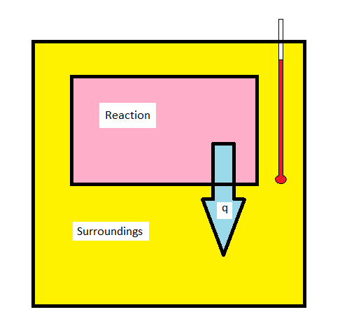
Calorimetry
- The techniques of calorimetrycan be used to measure \(q\) for a chemical reaction directly
- Calorimetry is based on the idea that if heat leaves the system it must enter the surroundings
- We measure the temperature change in the surroundngs, usually water
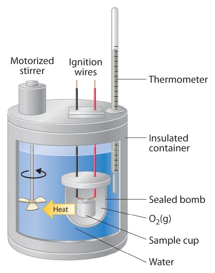
Bomb Calorimetry
- Bomb calorimetry is used mostly to measure the heat evolved in combustion reactions
"Water Equivalent" of a Bomb Calorimeter
- Bomb calorimeters are calibrated by carrying out a reaction with a known \(\Delta U_{rxn}\) - commonly the combustion of benzoic acid
- This calibration reaction allows the researcher to calculate the "water equivalent" (\(W\)) of the calorimeter
\[ W =\frac{n\,\Delta U_c + e_{wire} + e_{other}}{\Delta T} \]
- \(n\) is the number of moles of benzoic acid used
- \(\Delta U_c\) is the internal energy of combustion of benzoic acid (\( 3225.7\,\bfrac{kJ}{mol} \) at \(26^\circ C\))
- \(e_{wire}\) is the energy released in the combustion of the fuse wire
- \(e_{other}\) accounts for any other corrections
Using the "Water Equivalent"
- The "water equivalent" can be used to determine the \(\Delta U_c\) for an unknown reaction \[ \Delta U_c = \frac{W\,\Delta T-e_{wire}-e_{other}}{n_{sample}} \]
- The enthalpy of combustion can be found from the internal energy of combustion \[ \begin{eqnarray} \Delta H &=& \Delta U + \Delta (PV) \\ &=& \Delta U + RT\,\Delta n_{gas} \end{eqnarray} \]
- For benzoic acid \[ C_6H_5COOH(s) + 7.5O_2(g) \rightarrow 7CO_2(g) + 3H_2O(l) \] so \( \Delta n_{gas} = -0.5\,mol \)
Example 3.8
A student burned a \(0.7842\, g\) sample of benzoic acid (\(C_7H_6O_2\)) in a bomb calorimeter initially at \(25.0^\circ C\) and saw a temperature increase of \( 2.02^\circ C\). She then burned a \( 0.5348\, g\) sample of naphthalene (\(C_{10}H_8\)) (again from an initial temperature of \(25^\circ C\)) and saw a temperature increase of \( 2.24^\circ C\). From this data, calculate \(\Delta H_c\) for naphthalene (assuming \( e_{wire} \) and \( e_{other} \) are unimportant.)
Temperature Dependence of Enthalpy
- At constant pressure, \(dH=C_p\,dT\)
- For a temperature change we get \[ \Delta H = \int_{T_1}^{T_2} C_p\,dT \]
- If \(C_p\) is independent of temperature this reduces to \[ \Delta H = C_p\,\Delta T \]
Varying Heat Capacity
- A common emmpirical model can fit heat capacities over broad temperature ranges \[ C_p(T)=a+bT+\frac{c}{T^2} \]
- Plugging this into our enthalpy change equation yields \[ \begin{eqnarray} \Delta H &=& \int_{T_1}^{T_2} \left( a+bT+\frac{c}{T^2} \right)\,dT \\ &=& a \left(T_2-T_1\right)+\frac{b}{2}\left(T_2^2-T_1^2\right)-\frac{c}{3}\left(\frac{1}{T_2^3}-\frac{1}{T_1^3}\right) \end{eqnarray} \]
- For chemical reactions \[ \Delta H_{rxn}(T_2) = \Delta H_{rxn}(T_1) + \Delta C_p\,\Delta T \]
Empirical Parameters for the Temperature Dependence of \(C_p\)
| Substance | \(a\,(J\,mol^{-1}\,K^{-1})\) | \(b\,(J\,mol^{-1}\,K^{-2})\) | \(c\,(J\,mol^{-1}\,K)\) |
|---|---|---|---|
| \(C(gr)\) | \(16.86\) | \(4.77\times 10^{-3}\) | \(-8.54\times 10^5\) |
| \(CO_2(g)\) | \(44.22\) | \(8.79\times 10^{-3}\) | \(-8.62\times 10^5\) |
| \(H_2O(l)\) | \(75.29\) | \(0\) | \(0\) |
| \(N_2(g)\) | \(28.58\) | \(3.77\times 10^{-3}\) | \(-5.0\times 10^4\) |
| \(Pb(s)\) | \(22.13\) | \(1.172\times 10^{-2}\) | \(9.6\times 10^4\) |
Example 3.9
What is the molar enthalpy change for a temperature increase from \(273\, K\) to \(353\, K\) for \(Pb(s)\)?
Example 3.10
The enthalpy of formation of \( NH_3(g) \) is \( -46.11\,\bfrac{kJ}{mol} \) at \( 25^\circ C\). Calculate the enthalpy of formation at \( 100^\circ C \). Assuming heat capacities are independent of temperature.
| Substance | \(C_p\,(J\,mol^{-1}\,K^{-1})\) |
|---|---|
| \(N_2(g)\) | \(29.12\) |
| \(H_2(g)\) | \(28.82\) |
| \(NH_3(g)\) | \(35.06\) |
Reaction Enthalpies
- Reaction enthalpies are difficult to tabulate.
- We can use Hess' Law to simplify this
- We can use tabulated enthalpies to calculate the enthalpies of other reactions.
Example 3.11
Find \(\Delta H_{rxn}\) for the reaction \[ 2CO(g) + O_2(g) \rightarrow 2CO_2(g) \] given that \[ C(gr)+\frac{1}{2}O_2(g) \rightarrow CO(g) \;\;\; \Delta H = -110.53\,kJ \] \[ C(gr)+O_2(g) \rightarrow CO_2(g) \;\;\; \Delta H = -393.51\,kJ \]
Standard Enthalpy of Formation
- One problem with many thermodynamic state variables is that it is possible to measure changes but not absolute values
- It is therefore necessary to define a zero
- the standard enthalpy of formation of a pure element in its standard state is zero
The standard state of a substance is the most stable form of that substance at 1 atmosphere pressure and the specified temperature.
Standard Formation Reactions
- We measure and tabulate the standard formation reactions for compounds
- These reactions involve one of the substance in its standard state from elements in their standard states
- \(NaCl(s)\): \[ Na(s)+\frac{1}{2}Cl_2(g) \rightarrow NaCl(s)\;\;\; \Delta H_f^\circ = -411.2\bfrac{kJ}{mol} \]
- \(C_3H_8(g)\): \[ 3C(gr)+4H_2(g) \rightarrow C_3H_8(g)\;\;\; \Delta H_f^\circ = -103.8\bfrac{kJ}{mol} \]
- We can use Hess' Law with standard heats of formation
Alternation Use of Heats of Formation
- Because standard formation reactions begin with elements in their standard states we can simplify Hess' Law
- The reaction enthalpy can be calculated from the standard formation reaction enthalpy by \[ \Delta H_{rxn} =\sum_{products} \nu \cdot \Delta H_f^\circ - \sum_{reactants} \nu \cdot \Delta H_f^\circ \] where \(\nu\) is the stoichiometric coefficient of a species in the balanced chemical reaction
Ionization Reactions
- Formation of ions is seen throughout chemistry
- The enthalpy change to remove a single electron at \(0K\) from a species is defined as the ionization potential \[ M(g) \rightarrow M^+(g)+e^- \]
- The removal of subsequent electrons requires energies called the 2nd ionization potential, 3rd ionization potential, etc.
- Electon affinity is the enthalpy associated with the formation of negative ions \[ X(g) + e^- \rightarrow X^-(g) \] with \(-\Delta H(0K) \equiv 1^{st}\text{ electron affinity (EA)}\)
Average Bond Enthalpies
- Without standard formation enthalpies, we can estimate reaction enthalpies using average bond enthalpies - though this is not perfect
- A bond dissociation energy \(D\) is defined as \[ XY(g) \rightarrow X(g) + Y(g) \;\;\; \Delta H \equiv D(X-Y) \]
- Using this we can estimate the reaction enthalpy \[ \Delta H_{rxn} = \sum \left(\text{bonds broken}\right) - \sum \left(\text{bonds formed}\right) \]
Example 3.12
Estimate the reaction enthalpy for the combustion of ethanol \[ C_2H_5OH(g) + O_2(g) \rightarrow 2CO_2(g) + H_2O(g) \] using
| Bond | Average Bond Energy (kJ/mol) |
|---|---|
| C-H | 413 |
| C-C | 348 |
| C-O | 358 |
| O=O | 495 |
| C=O | 799 |
| O-H | 463 |
The Born-Haber Cycle
- It is handy to construct thermodynamic cycles to help understand thermodynamics
- The Born-Haber Cycle is used to describe the formation of an ionic solid
- For the formation of \(Na(s)+\frac{1}{2}Cl_2(g)\rightarrow NaCl(s)\): \[ \begin{eqnarray} Na(s)\rightarrow Na(g) &\;\;\;& \Delta H_{sub}(Na) \\ Na(g)\rightarrow Na^+(g)+e^- &\;\;\;& 1^{st}IP(Na) \\ \frac{1}{2}Cl_2(g)\rightarrow Cl(g) &\;\;\;& \frac{1}{2}D(Cl-Cl) \\ Cl(g) + e^-\rightarrow Cl^-(g) &\;\;\;& 1^{st}EA(Cl) \\ Na^+(g) + Cl^-(g) \rightarrow NaCl(s) &\;\;\;& \Delta H_{lat}(NaCl) \end{eqnarray} \]
Example 3.13
Find \(\Delta H_f\) for \(KBr\) given the following data: \[ \begin{eqnarray} K(s)\rightarrow K(g) &\;\;\;& \Delta H_{sub}(K)=89\bfrac{kJ}{mol} \\ Br_2(l)\rightarrow Br_2(g) &\;\;\;& \Delta H_{vap}=31\bfrac{kJ}{mol} \\ Br_2(g)\rightarrow 2Br(g) &\;\;\;& D(Br-Br)=193\bfrac{kJ}{mol} \\ K(g)\rightarrow K^+(g)+e^- &\;\;\;& 1^{st}IP(K)=419\bfrac{kJ}{mol} \\ Br(g) + e^-\rightarrow Br^-(g) &\;\;\;& 1^{st}EA(Br)=194\bfrac{kJ}{mol} \\ K^+(g) + Br^-(g) \rightarrow KBr(s) &\;\;\;& \Delta H_{lat}(KBr)=675\bfrac{kJ}{mol} \end{eqnarray} \]
Born-Haber Cycle Graphically
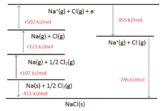
/