Chemical Kinetics 2

Shaun Williams, PhD

Reaction Mechanisms

A reaction mechanism is a set of elementary steps that when taken together define a chemical pathway that connects the reactants to the products.
An elementary reaction is one that proceeds by a single process
- molecular (or atomic) decomposition
- molecular collision
The molecularity of an elementary reaction defines the order of the rate law for that reaction step.

Molecularity of Elementary Reactions

Unimolecular elementary reactions have a single reactant \[ A\rightarrow \text{products} \]
Bimolecular elementary reaction involve the collision of two reactants \[ A+B \rightarrow \text{products} \]
Termolecular elementary reactions involve the collision of three reactants (these are rare for obvious reasons) \[ A+B+C \rightarrow \text{products} \]
Another, more common form of termolecular elementary reactions involve two rapid steps \[ A+B \rightarrow AB^* \] \[ AB^* + C \rightarrow AB+C^* \]

The Requirements of a Reaction Mechanism

A valid reaction mechanism must satisfy three important criteria

The sum of the steps must yield the overall stoichiometry of the reaction.
The mechanism must be consistent with the observed kinetics for the overall reaction.
The mechanism must account for the possibility of any observed side products formed in the reaction.

Example 12.1

For the reaction \[ A+B \rightarrow C \] is the following proposed mechanism valid? \[ A+A \xrightarrow{k_1} A_2 \] \[ A_2 + B \xrightarrow{k_2} C+A \]

Concentration Profiles for Some Simple Mechanisms

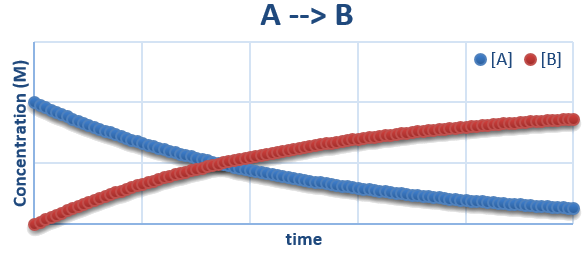
\(A \rightarrow B\)

If this reaction is a single unimolecular elementary step then it can be writted as \[ A \xrightarrow{k_1} B \]
Since it is an elementary step we can easily write the rate laws for it \[ \frac{d[A]}{dt} = -k_1[A] \] \[ \frac{d[B]}{dt} = +k_1[A] \]

A plot of \(A \rightarrow B\)

As the concentration of A decreases there is an eqivalent increase in the concentration of B.

\( A \rightleftharpoons B \)

The rate of change of the A and B will depend on both the forward and the backward reactions \[ A \xrightarrow{k_1} B \] \[ B \xrightarrow{k_{-1}} A \] or more typically \[ A \xrightleftharpoons{k_1}{k_{-1}} B \]
The rate of change of concentration of A and B are \[ \frac{d[A]}{dt} = -k_1[A] + k_{-1}[B] \] \[ \frac{d[B]}{dt} = +k_1[A] - k_{-1}[B] \]

A plot of \(A \rightleftharpoons B\)

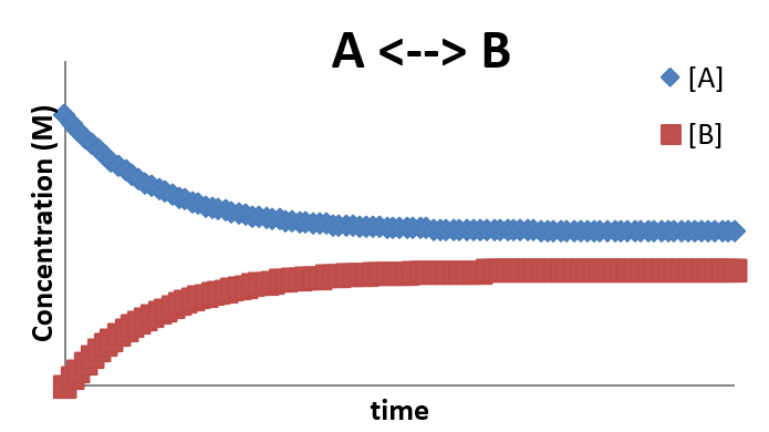
As the concentration of A decreases there is an eqivalent increase in the concentration of B. Over time, the concentration of each species levels out as the system reaches equilibrium.

This profile illustrates that even after the system achieves equilibrium, the forward and reverse reactions are still taking place.
This is the nature of a dynamic equilibrium

At Equilibrium

At equilibrium, the rate of formation of A and the rate of formation of B must be equal to zero \[ \frac{d[A]}{dt} = -k_1[A] + k_{-1}[B] = 0 \] \[ k_1[A] = k_{-1}[B] \] \[ \frac{k_1}{k_{-1}} = \frac{[B]}{[A]} \]
So, the ratio of \(k_1\) to \(k_{-1}\) gives the value of the equilibrium constant, \(K_{eq}=\frac{[\text{products}]}{[\text{reactants}]} \)

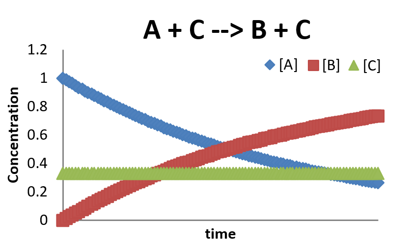
\( A+C \rightarrow B+C \)

Some reactions require a catalyst to mediate the reaction
Catalysts are species that must be added (not formed as intermediates)
Catalysts show up in the mechanism, usually in an early step
Catalysts end up as part of the rate law
Catalysts are reformed later so they don't appear in the overall reaction stoichiometry
If the reaction \(A\rightarrow B\) is aided by a catalyst \(C\) then \[ A+C \rightarrow B+C \]

Kinetics of \(A+C \rightarrow B+C \)

The rate of change of the concentrations is \[ \frac{d[A]}{dt} = -k[A][C] \] \[ \frac{d[B]}{dt} = +k[A][C] \] \[ \frac{d[C]}{dt} = -k[A][C] + k[A][C] = 0 \]

As the concentration of A decreases there is an eqivalent increase in the concentration of B. The concentration of the catalyst C is constant in time.

Final Anaylsis of \( A+C \rightarrow B+C \)

This is a very simplified picture of reaction calaysis
Generally, catalyzed reaction occur in at least two steps \[ A+B \rightarrow AC \] \[ AC \rightarrow B+C \]
Later we will see how to handle this

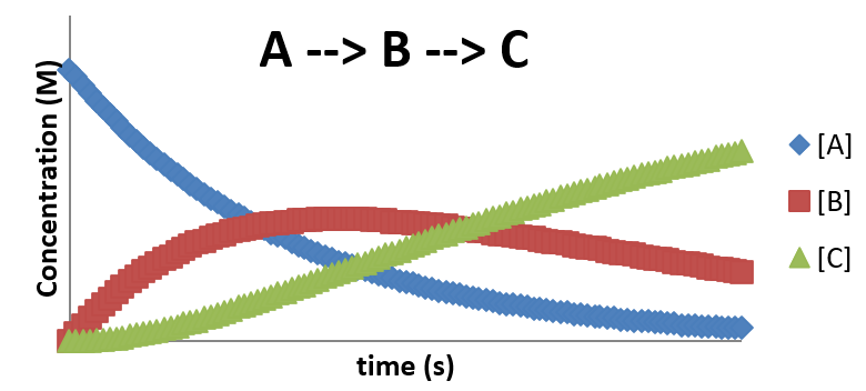
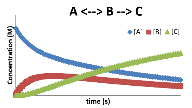
\( A \rightarrow B \rightarrow C \)

This mechanism features the formation of an intermediate
Intermediates are species that are formed in one step and used in a later step
Intermediates do not appeat in the reactions's stoichiometry
Unlike catalysts, intermediates are not added to the reaction, but are created during the reaction.
This reaction, \( A \xrightarrow{k_1} B \xrightarrow{k_2} C \) would have rate laws \[ \frac{d[A]}{dt} = -k_1[A] \] \[ \frac{d[B]}{dt} = k_1[A] - k_2[B] \] \[ \frac{d[C]}{dt} = k_2[B] \]

A plot of \(A \rightarrow B \rightarrow C\)

The initial fall in the concentration of A is mirrored by an initial rise in the concentration of B. As the concentration of B rises we see a rise in the concentration of C. The concentration of B reaches a maximum and the begins to drops.

\(A \rightleftharpoons B \rightarrow C \)

In many cases, the formation of an intermediate involves reversible step
This step is sometimes called a pre-equilibrium step since it often will establish a near equilibrium while the reaction progresses
This reaction can be broken down into two mechanistic steps \[ A \xrightleftharpoons{k_1}{k_{-1}} B \;\;\text{and}\;\; B \xrightarrow{k_2} C \] \[ \frac{d[A]}{dt} = -k_1[A]+k_{-1}[B] \] \[ \frac{d[B]}{dt} = k_1[A]-k_{-1}[B] -k_2[B] \] \[ \frac{d[C]}{dt} = k_2[B] \]

A plot of \(A \rightleftharpoons B \rightarrow C\)

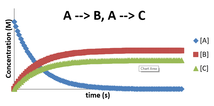
As the concentration A falls, the concentration of B rapidly rises to a maximum and then levels off and then declines slowly in time. As the concentration of B increases the concentration of C also increases and it continues to increase even after the concentration of B begins to fall.

\(A \rightarrow B\) and \(A \rightarrow C\)

There are many cases where a reactant can follow pathways to different products
These pathways compete with each other
A example is the following simple mechanism \[ A \xrightarrow{k_1} B \] \[ A \xrightarrow{k_2} C \] \[ \frac{d[A]}{dt} = -k_1[A]-k_2[A] \] \[ \frac{d[B]}{dt} = k_1[A] \] \[ \frac{d[C]}{dt} = k_2[A] \]

A plot of \(A \rightarrow B\) and \(A\rightarrow C\)

As the concentration A falls, the concentration of both B and C rise.

The Connection Between Reaction Mechanisms and Reaction Rate Laws

Chemical kinetics gives us insights into the actual reaction pathways (mechanisms) that are followed
Analyzing a reaction mechanism to determine the type of rate law that is consistant (or inconsistant) with a specific mechanism is important

An example: \(A+B\rightarrow C\)

\[ \underbrace{A+A\xrightarrow{k_1}A_2}_{\text{step 1}} \] \[ \underbrace{A_2+B\xrightarrow{k_2} C}_{\text{step 2}} \]
\[ \underbrace{A\xrightarrow{k_1}A^*}_{\text{step 1}} \] \[ \underbrace{A^*+B\xrightarrow{k_2} C}_{\text{step 2}} \]

Analysis of our example

The first rate law will predict that the reaction should be second order in A.
The second rate law will predict that the reaction should be first order in A.
Based on the experimentally determined rate law's order, you can rule out one of these mechanisms.
In order to analyze mechanisms and predict rate laws, we need some tools...

The Rate Determining Step Approximation

The rate determining step approximation states that a mechanism can proceed no faster than its slowest step
For example: \[ \underbrace{A+A\xrightarrow{k_1}A_2}_{\text{slow}} \;\;\text{and then} \;\; \underbrace{A_2+B\xrightarrow{k_2} C}_{\text{fast}} \]
The rate determining step approximation says that the rate should be determined by the slow initial step \[ \frac{d[C]}{dt}=k_1[A]^2 \]

The Other Mechanism

We can do the same for the other proposed mechanism \[ \underbrace{A\xrightarrow{k_1}A^*}_{\text{slow}} \] \[ \underbrace{A^*+B\xrightarrow{k_2} C}_{\text{fast}} \] so the rate law would be \[ \frac{d[C]}{dt} = k_1[A] \]

The Steady-State Approximation

This is one of the most common approximations
This approximation can be applied to the rate of change of concentration of a highly reactive (short lived) intermediate that holds a constant value over a long period of time
The advantage is that for such an intermediate \(I\) \[ \frac{d[I]}{dt} = 0 \]

Our First Proposed Mechanism Again

In our mechanism \[ A+A\xrightarrow{k_1}A_2 \] \[ A_2+B\xrightarrow{k_2} C \] \(A_2\) is an intermediate
So, using the steady state approximation \[ \frac{d[A_2]}{dt} = k_1[A]^2-k_2[A_2][B] \approx 0 \]
Thus \[ [A_2] \approx \frac{k_1[A]^2}{k_2[B]} \]

Further Simplification

\( [A_2] \approx \frac{k_1[A]^2}{k_2[B]} \)

We can use that result to simplify our rate of product production \[ \begin{eqnarray} \frac{d[C]}{dt} &=& k_2[A_2][B] \\ &=& k_2 \left( \frac{k_1[A]^2}{k_2[B]} \right)[B] \\ &=& k_1[A]^2 \end{eqnarray} \]

Our Second Proposed Mechanism Again

In our mechanism \[ A\xrightarrow{k_1}A^* \] \[ A^*+B\xrightarrow{k_2} C \] \(A^*\) is an intermediate
So, using the steady state approximation \[ \frac{d[A^*]}{dt} = k_1[A]-k_2[A^*][B] \approx 0 \]
Thus \[ [A^*] \approx \frac{k_1[A]}{k_2[B]} \]

Further Simplification to the Second

\( [A^*] \approx \frac{k_1[A]}{k_2[B]} \)

We can use that result to simplify our rate of product production \[ \begin{eqnarray} \frac{d[C]}{dt} &=& k_2[A^*][B] \\ &=& k_2 \left( \frac{k_1[A]}{k_2[B]} \right)[B] \\ &=& k_1[A] \end{eqnarray} \]

Example 12.2

Use the steady-state approximation to derive the rate law for this reaction \[ \chem{2N_2O_5 \rightarrow 4NO_2 + O_2} \] assuming it follows the following three-step mechanism: \[ \chem{N_2O_5} \xrightleftharpoons{k_f}{k_b} \chem{NO_2 + NO_3} \] \[ \chem{NO_3 + NO_2} \xrightarrow{k_2} \chem{NO + NO_2 + O_2} \] \[ \chem{NO_3 + NO} \xrightarrow{k_3} \chem{2NO_2} \]

The Equilibrium Approximation

As mentioned, in many cases, the formation of an intermediate involves a reversible step
If the intermediate can reform reactants with a significant probability compared to forming products then we can utilize the equilibrium approximation

An Equilibrium Approximation Mechanism

Consider the following mechanism \[ A+B \xrightleftharpoons{k_1}{k_{-1}} AB \] \[ AB \xrightarrow{k_2} C \]
Due to the equilibrium, the steady state approximation would be combersome
If the initial step is assumed to achieve equilibrium then \[ k_1[A][B]=k_{-1}[AB] \] \[ [AB]=\frac{k_1[A][B]}{k_{-1}} \]

Plugging in Our Approximation

\( [AB]=\frac{k_1[A][B]}{k_{-1}} \)

We can now plug our approximation value into the rate of formation of our product \[ \begin{eqnarray} \frac{d[C]}{dt} &=& k_2[AB] \\ &=& k_2 \left( \frac{k_1[A][B]}{k_{-1}} \right) \\ &=& \frac{k_1k_2 [A][B]}{k_{-1}} \end{eqnarray} \]

Example 12.3

Given the following mechanism, apply the equilibrium approximation to the first step to predict the rate law suggested by the mechanism. \[ A+A \xrightleftharpoons{k_1}{k_{-1}} A_2 \] \[ A_2 + B \xrightarrow{k_2} C+A \]

Another Interesting Case

Let's look at the following mechanism for the reaction \( A+2B\rightarrow 2C \) \[ A+B \xrightleftharpoons{k_1}{k_{-1}} I+C \] \[ I+B \xrightarrow{k_2} C \]
Using the equilibrium approximation on \(I\) we find that \[ k_1[A][B] = k_{-1}[I][C] \;\;\Rightarrow\;\; [I]\approx \frac{k_1[A][B]}{k_{-1}[C]} \]

Simplifying Our New Case

\( [I]\approx \frac{k_1[A][B]}{k_{-1}[C]} \)

We can substitute this into our expression for the rate of product formation \[ \begin{eqnarray} \frac{d[C]}{dt} &=& k_2[I][B] \\ &=& k_2 \left( \frac{k_1[A][B]}{k_{-1}[C]} \right) [B] \\ &=& \frac{k_1k_2[A][B]}{k_{-1}[C]} = k'\frac{[A][B]}{[C]} \end{eqnarray} \] where \( k'=\frac{k_1k_2}{k_{-1}} \)
This rate law is first order in A and B but is negative 1 order in C.

The Lindemann Mechanism

The Lindemann Mechanism is useful to demonstrate our kinetics techniques
In the mechanism, a reactant is collisionally activated to an energetic state
That energetic state can then return to reactants or form the products.
Consider the following mechanism \[ A+A \xrightleftharpoons{k_1}{k_{-1}} A^* + A \] \[ A^* \xrightarrow{k_2} P \]

Applying the Steady State Approximation

If we apply the steady state approximation to our intermediate \(A^*\) we find that \[ \frac{d[A^*]}{dt} = k_1[A]^2-k_{-1}[A^*][A]-k_2[A^*]\approx 0 \] \[ [A^*] \approx \frac{k_1[A]^2}{k_{-1}[A]+k_2} \]
Substituting that into our rate of product formation \[ \begin{eqnarray} \frac{d[P]}{dt} &=& k_2[A^*] \\ &=& k_2 \left( \frac{k_1[A]^2}{k_{-1}[A]+k_2} \right) = \frac{k_1k_2[A]^2}{k_{-1}[A]+k_2} \end{eqnarray} \]

Analyzing the Result

\( \frac{d[P]}{dt}= \frac{k_1k_2[A]^2}{k_{-1}[A]+k_2} \)

In the limit that \(k_{-1}[A]\ll k_2\) then \[ \frac{d[P]}{dt}= \frac{k_1k_2[A]^2}{k_2}=k_1[A]^2 \]
In the limit that \(k_{-1}[A]\gg k_2\) then \[ \frac{d[P]}{dt}= \frac{k_1k_2[A]^2}{k_{-1}[A]}=\frac{k_1k_2[A]}{k_{-1}} \]

Third Body Collisions

Sometimes a third-body collision is provided by an inert species \(M\) (such as argon in a gas reaction)
In this case the mechanism could be \[ A+M \xrightleftharpoons{k_1}{k_{-1}} A^* + M \] \[ A^* \xrightarrow{k_2} P \]
We can again use the stedy state approximation on \(A^*\) \[ \frac{d[A^*]}{dt} = k_1[A][M]-k_{-1}[A^*][M]-k_2[A^*]\approx 0 \] \[ [A^*] \approx \frac{k_1[A][M]}{k_{-1}[M]+k_2} \]

Rate of Product in Third Body Collisions

\( [A^*] \approx \frac{k_1[A][M]}{k_{-1}[M]+k_2} \)

We can now insert this into our rate of product formation reaction \[ \begin{eqnarray} \frac{d[P]}{dt} &=& k_2[A^*] \\ &=& k_2 \frac{k_1[A][M]}{k_{-1}[M]+k_2} = \frac{k_1k_2[A][M]}{k_{-1}[M]+k_2} \end{eqnarray} \]
If the concentration of \(M\) is constant then we can define a new effective rate constant, \(k_{uni}\) \[ k_{uni} = \frac{k_1k_2[M]}{k_{-1}[M]+k_2} \] \[ \frac{d[P]}{dt} = k_{uni}[A] \]

Analysis of the Effective Rate Constant

\( k_{uni} = \frac{k_1k_2[M]}{k_{-1}[M]+k_2} \)

We can get very useful information about the individual steps we measure \(k_{uni}\) at various concentration of the third body collider \[ \frac{1}{k_{uni}} = \frac{k_{-1}[M]+k_2}{k_1k_2[M]} \] \[ \frac{1}{k_{uni}} = \frac{k_{-1}}{k_1k_2} + k_2\left(\frac{1}{[M]}\right) \]
So, if we plot \(\frac{1}{k_{uni}}\) versus \(\frac{1}{[M]}\) we will get a straight line and
- The slope will be \(k_2\)
- The intercept will be \(\frac{k_{-1}}{k_1k_2}\)

The Michaelis-Menten Mechanism

The Michaelis-Menten mechanism is one which many enzyme mitigated reactions follow
An enzyme (\(E\)) and a substrate (\(S\)) connect to form an enzyme-substrate complex (\(ES\))
The enzyme-substrate complex degrades to form the product (\(P\))
Overall, \(S\rightarrow P\) \[ E+S \xrightleftharpoons{k_1}{k_{-1}} ES \] \[ ES \xrightarrow{k_2} P+E \]

Analyzing Michaelis-Menten: The Beginning

We first apply the equilibrium approximation to the first step \[ k_1[E][S] \approx k_{-1} [ES] \]
Using mass conservation on the enzyme \[ [E]_0 = [E]+[ES] \;\;\Rightarrow\;\; [E]=[E]_0-[ES] \]
Plugging this into our equilibrium approximation \[ k_1\left( [E]_0-[ES] \right)[S] = k_{-1} [ES] \] \[ k_1[E]_0[S]-k_1[ES][S] = k_{-1} [ES] \] \[ k_1[E]_0[S] = k_1[ES][S] + k_{-1} [ES] = \left(k_1[S]+k_{-1}\right)[ES] \] \[ \frac{k_1[E]_0[S]}{k_1[S]+k_{-1}}=[ES] \]

Analyzing Michaelis-Menten: Continuing

\( [ES]=\frac{k_1[E]_0[S]}{k_1[S]+k_{-1}} \)

Plugging this into the rate of product formation \[\begin{eqnarray} \frac{d[P]}{dt} &=& k_2[ES] \\ &=& k_2 \left( \frac{k_1[E]_0[S]}{k_1[S]+k_{-1}} \right) \\ &=& \frac{k_1k_2[E]_0[S]}{k_1[S]+k_{-1}} \end{eqnarray}\]
Multiply the top and bottom by \(\frac{1}{k_1}\) \[ \frac{d[P]}{dt} = \frac{k_2[E]_0[S]}{[S]+\frac{k_{-1}}{k_1}} \]

Analyzing Michaelis-Menten: Finishing

\( \frac{d[P]}{dt} = \frac{k_2[E]_0[S]}{[S]+\frac{k_{-1}}{k_1}} \)

The ratio \(\frac{k_{-1}}{k_1}\) is the equilibrium constant that describes the dissociation of the enzyme-substrate complex, \(K_d\)
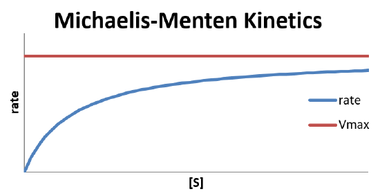
The value \(k_2[E]_0\) is the maximum rate, \(V_{max}\)
This means that we can write our equation as \[ \frac{d[P]}{dt} = \text{rate} = \frac{V_{max}[S]}{K_d+[S]} \]

Analyzing Michaelis-Menten with Steady-State Approximation: The Beginning

Alternatively we can derive our expression using the steady-state approximation on \(ES\) \[ \frac{d[ES]}{dt} = k_1[E][S]-k_{-1}[ES] - k_2[ES]\approx 0 \] \[ [ES]=\frac{k_1[E][S]}{k_{-1}+k_2} = \frac{[E][S]}{K_m} \] where \(K_m=\frac{k_{-1}+k_2}{k_1}\) is the Michaelis constant.
Plugging that is we find that \[ \frac{d[P]}{dt} = \frac{V_{max}[S]}{K_m+[S]} \]

Plot of Michaelis-Menten Kinetics

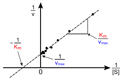
A plot of the rate of the reaction versus concentration of substrate. Vmax is constant and as the amount of substrate is increased, the rate of the reaction increase and approaches Vmax.

Lineweaver-Burk Plot

Michaelis-Menten studies will measure the rate of the reaction as a function of substrate concentration
We can rearrange our rate equation some that it becomes linear \[ \frac{1}{\text{rate}}=\frac{K_m+[S]}{V_{max}[S]} \] \[ \frac{1}{\text{rate}}=\frac{K_m}{V_{max}}\frac{1}{[S]}+\frac{1}{V_{max}} \]

A Lineweaver-Burk Plot Example

A plot of 1 over rate versus 1 over substrate concentration is linear. The slope of the line is Km over Vmax and the y-intercept is -1 over Vmax.

Chain Reactions

A large number of reaction proceed through a series of steps that can collectively be classified as a chain reaction
The reaction steps can be classified as
- initiation step - a step that creates the intermediates from stable species
- propagation step - a step that consumes an intermediate, but creates a new one
- termination step - a step that consumes intermediates without creating new ones
These types of reations are very common when the interemediates involved are radiacals

Chain Reaction Example

Consider the reaction \[ H_2+ Br_2 \rightarrow 2HBr \]
The observed rate law for this reaction is \[ \text{rate} = \frac{k[H_2][Br_2]^\frac{3}{2}}{[Br_2]+k'[HBr]} \]

Chain Reaction Example Mechanism

The proposed mechanism is \[ Br_2 \xrightleftharpoons{k_1}{k_{-1}} 2Br\cdot \] \[ 2Br\cdot + H_2 \xrightleftharpoons{k_2}{k_{-2}} HBr + H\cdot \] \[ H\cdot + Br_2 \xrightarrow{k_3} HBr + Br\cdot \]

Mechanism Analysis

The change in concentrations of the intermediates can be written and the steady state approximation applied \[ \frac{d[H\cdot]}{dt} = k_2[Br\cdot][H_2]-k_{-2}[HBr][H\cdot]-k_3[H\cdot][Br_2]\approx 0 \] \[ \begin{align} \frac{d[Br\cdot]}{dt} = 2k_1[Br_2]&-2k_{-1}[Br\cdot]^2-k_2[Br\cdot][H_2] \\ &+k_{-2}[HBr][H\cdot]+k_3[H\cdot][Br_2] \approx 0 \end{align} \]
Adding these two expression cancels the terms involving \(k_2\), \(k_{-2}\), and \(k_3\) \[ 2k_1[Br_2]-2k_{-1}[Br\cdot]^2=0 \]

Mechanism Analysis Continued

Solving the equation from \(Br\cdot\) \[ [Br\cdot] = \sqrt{\frac{k_1[Br_2]}{k_{-1}}} \]
This can be substituted into an expression for the \(H\cdot\) that is made by solving the steady state expression for \( \frac{d[H\cdot]}{dt}\) \[ [H\cdot] = \frac{k_2[Br\cdot][H_2]}{k_{-2}[HBr]+k_3[Br_2]} = \frac{k_2\sqrt{\frac{k_1[Br_2]}{k_{-1}}}[H_2]}{k_{-2}[HBr]+k_3[Br_2]} \]

Mechanism Analysis: Simplifying

We can substitute are expression for \([H\cdot]\) and \([Br\cdot]\) into the rate of production of \(HBr\) \[ \begin{eqnarray} \frac{d[HBr]}{dt} &=& k_2[Br\cdot][H_2]+k_3[H\cdot][Br_2]-k_{-2}[H\cdot][HBr] \\ &=& k_2\sqrt{\frac{k_1[Br_2]}{k_{-1}}}[H_2]+k_3\left( \frac{k_2\sqrt{\frac{k_1[Br_2]}{k_{-1}}}[H_2]}{k_{-2}[HBr]+k_3[Br_2]} \right)[Br_2] \\ && -k_{-2}\left( \frac{k_2\sqrt{\frac{k_1[Br_2]}{k_{-1}}}[H_2]}{k_{-2}[HBr]+k_3[Br_2]} \right)[HBr] \end{eqnarray} \]

Mechanism Analysis: Simplifying This Time

Let's try to actually simplify the expression \[ \text{rate} = k_2\sqrt{\frac{k_1[Br_2]}{k_{-1}}}[H_2] \left[ 1+\frac{k_3[Br_2]}{k_{-2}[HBr]+k_3[Br_2]}-\frac{k_{-2}[HBr]}{k_{-2}[HBr]+k_3[Br_2]} \right] \] \[ \text{rate} = k_2\sqrt{\frac{k_1[Br_2]}{k_{-1}}}[H_2] \left[ \begin{array}{l} \frac{k_{-2}[HBr]+k_3[Br_2]}{k_{-2}[HBr]+k_3[Br_2]} \\ +\frac{k_3[Br_2]}{k_{-2}[HBr]+k_3[Br_2]} \\ -\frac{k_{-2}[HBr]}{k_{-2}[HBr]+k_3[Br_2]} \end{array} \right] \]

Mechanism Analysis: Maybe this time!

Now we can combine and start canceling some terms \[ \text{rate} = k_2\sqrt{\frac{k_1[Br_2]}{k_{-1}}}[H_2] \left[ \frac{k_{-2}[HBr]+k_3[Br_2]+k_3[Br_2]-k_{-2}[HBr]}{k_{-2}[HBr]+k_3[Br_2]} \right] \] \[ \text{rate} = k_2\sqrt{\frac{k_1[Br_2]}{k_{-1}}}[H_2] \left[ \frac{2k_3[Br_2]}{k_{-2}[HBr]+k_3[Br_2]} \right] \] \[ \text{rate} = \frac{2k_2k_3\sqrt{\frac{k_1}{k_{-1}}}[H_2][Br_2]^\frac{1}{2}}{k_{-2}[HBr]+k_3[Br_2]} \]

Mechanism Analysis: A Final Simplification

\( \text{rate} = \frac{2k_2k_3\sqrt{\frac{k_1}{k_{-1}}}[H_2][Br_2]^\frac{1}{2}}{k_{-2}[HBr]+k_3[Br_2]} \)

Doing a little algebra we find that \[ \text{rate} = \frac{2k_2k_3\sqrt{\frac{k_1}{k_{-1}}}[H_2][Br_2]^\frac{1}{2}}{\frac{k_{-2}}{k_3}[HBr]+[Br_2]} = \frac{k[H_2][Br_2]^\frac{1}{2}}{k'[HBr]+[Br_2]} \] where \(k'=\frac{k_{-2}}{k_3}\) and \(k=2k_2k_3\sqrt{\frac{k_1}{k_{-1}}}\)
This matches the experimental rate law

Catalysis

There are many examples of reactions that involve catalysis
One important example is from the environments, the catalytic decomposition of ozone \[ O_3 + O \rightarrow 2O_2 \]
This reaction can be catalyzed by atomic chlorine

Mechanism of Ozone Decomposition

The mechanism for the catalytic decomposition of ozone is \[ O_3 + Cl \xrightarrow{k_1} ClO+O_2 \] \[ ClO+O \xrightarrow{k_2} Cl + O_2 \]
The rate of change of the intermediate (\(ClO\)) concentration is given by \[ \frac{d[ClO]}{dt} = k_1 [O_3][Cl] - k_2[ClO][O] \]

Analysis of Ozone Decomposition Mechanism

Applying the steady state approximation to the intermediate \[ [ClO] = \frac{k_1[O_3][Cl]}{k_2[O]} \]
The rate of production of the product, \(O_2\), is \[ \frac{d[O_2]}{dt} = k_2[O_3][Cl]+k_2[ClO][O] = k_2[O_3][Cl]+k_2\left( \frac{k_1[O_3][Cl]}{k_2[O]} \right)[O] \] \[ \frac{d[O_2]}{dt} = k_2[O_3][Cl]+ k_1[O_3][Cl] = \left(k_1+k_2\right)[O_3][Cl] \]

Schematic of Ozone Decomposition

Ozone reacts with chlorine atoms to create ClO and O2 with the O2 leaving. The ClO reacts with atomic oxygen to create more O2, which leaves, and reforming chlorine atoms.

Oscillating Reactions

Most reaction convert reactant to products in a smooth process
Some reactions show irregular behavior
One particular phenomenon is that of oscillating reactions where the reactant concentrations rise and fall as the reaction progresses
One way this happens is when the products of the reaction catalyze the reaction - this is called autocatalysis

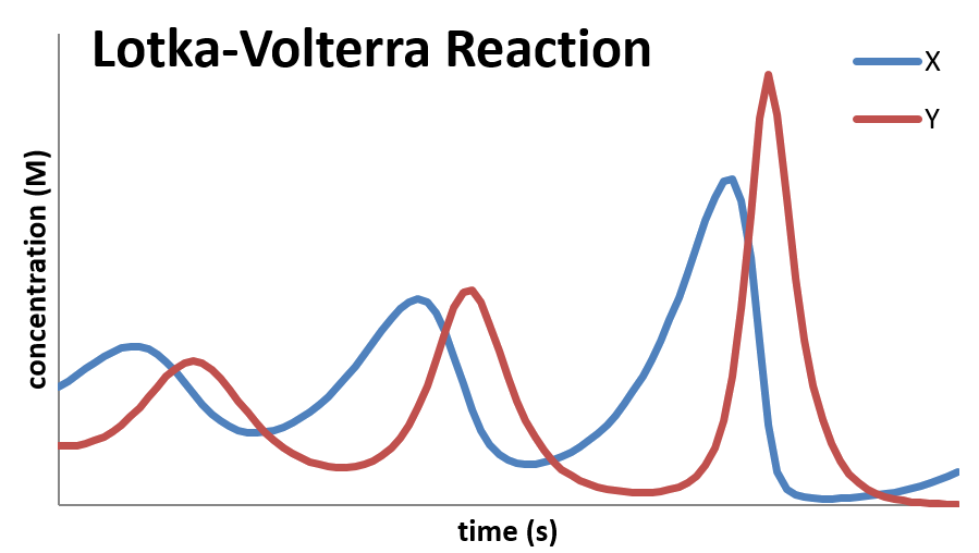
The Lotka-Voltera Mechanism

An example of an autocatalyzed mechanism is the Lotka-Voltera mechanism \[ A+X \xrightarrow{k_1} X+X \] \[ X+Y \xrightarrow{k_2} Y+Y \] \[ Y \xrightarrow{k_3} B \]
In this reaction, the concentration of A is held constant by continually adding it to the reaction mixture
The first step is autocatalyzed so it speeds up in over time... as it the second step

Schematic of Lotka-Voltera Mechanism

A plot of concentration versus time. As the reaction begins we see a rise to a maximum of A. As it fall we see a rise to a maximum of B. As B fall we see a second rise to a higher concentration of A. The concentration of A then falls as the concentration of B rises to an even higher concentration. The process continues until reactants are exhausted.