Chemical Kinetics 1
Shaun Williams, PhD
Reaction Rate
- The rate of a chemical reaction (or reaction rate) is the time needed for a change in concentration to occur.
- The problem with this is that both the reactants and the products can be changing their concentrations
- Plus, there are conplications due to stoichiometry issues
- For the general reaction equation: \(aA+bB\rightarrow cC+dD\) the reaction rate is \[ \text{rate}=-\frac{1}{a}\frac{\Delta [A]}{dt}=-\frac{1}{b}\frac{\Delta [B]}{dt} = +\frac{1}{c}\frac{\Delta [C]}{dt}=+\frac{1}{d}\frac{\Delta [D]}{dt} \] or \[ \text{rate}=-\frac{1}{a}\frac{d [A]}{dt}=-\frac{1}{b}\frac{d [B]}{dt} = +\frac{1}{c}\frac{d [C]}{dt}=+\frac{1}{d}\frac{d [D]}{dt} \]
Example 11.1
Under a certain set of conditions, the rate of the reaction \[ N_2+3H_2\rightarrow 2NH_3 \] the reaction rae is \(6.0\times 10^{-4}\bfrac{M}{s}\). Calculate the time-rate of change for the concentration of \(N_2\), \(H_2\), and \(NH_3\).
Measuring Reaction Rates
- There are several ways of measuring chemical reaction rates
- Commonly we use spectrophotometry to monitor the concentration of species that absorb light
- We prefer to measure the appearance of the product rather than disappearance of the reactants - background interference issue
- We can, however, get highly accurate measurements either way
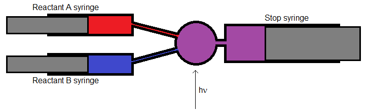
The Stopped-Flow Method
- The stopped-flow method involves using flow control (syringes or valves) to control the flow of reactants into a mixing chamber
- The reaction mixture can them be probed with light
Other Methods
- Some methods dependon measuring the initial rate of the reaction, which can have a lot of experimental uncertainty
- Other measures require a huge number of time and concentration data
- These later designs tend to produce more reliable results since their smooth away fluctuations of concentration in time.
- We will discuss these methods more later.
Rate Laws
- A rate law is any mathematical relationship that relates concentration of reactant or product to time in a chemical reaction
- Rate laws can be expressed in either derivative or integrated forms
- One of the most common general forms of a rate law for the reaction \(A+B\rightarrow \text{products}\) is \[ \text{rate}=k[A]^\alpha [B]^\beta \] where \(k\), \(\alpha\), and \(\beta\) are experimentally determined.
More Complicated Forms
- Rate laws are not always are simplistic as what we just saw
- Some rate laws may have powers that are not integers, for example \[ \text{rate}=k[A]^\alpha [B]^\bfrac{1}{2} \]
- Some rate laws may include the concentration of products \[ \text{rate}=\frac{k[A]^\bfrac{1}{2}[B]}{[P]} \]
- In some cases, the concentration of a catalyst or enzyme is important
- Many enzyme mitigated reactions in biological systems follow the Michaulis-Menten rate law \[ \text{rate}=\frac{V_{max}[S]}{K_m+[S]} \]
Order
- Consider those cases where the rate law can be expressed in the form \[ \text{rate}=k[A]^\alpha [B]^\beta [C]^\gamma \]
- We say that the reaction is of \(\alpha\) order in \(A\), \(\beta\) order in \(B\), and \(\gamma\) order in \(C\).
- Additionally, the reaction is said to be \(\alpha+\beta+\gamma\) order overall.
- In all cases: the reaction with respect to reactants and products must be determined experimentally
- Stoichiometry can not be used to predict the form of the rate law
Example Rate Laws
| Rate Law | Order in A | Order in B | Order in C | Overall Order |
|---|---|---|---|---|
| \( \text{rate}= k \) | 0 | 0 | 0 | 0 |
| \( \text{rate}= k[A] \) | 1 | 0 | 0 | 1 |
| \( \text{rate}= k[A]^2 \) | 2 | 0 | 0 | 2 |
| \( \text{rate}= k[A][B] \) | 1 | 1 | 0 | 2 |
| \( \text{rate}= k[A]^2[B] \) | 2 | 1 | 0 | 3 |
| \( \text{rate}= k[A][B][C] \) | 1 | 1 | 1 | 3 |
| \( \text{rate}= k[A][B]^\frac{1}{2} \) | 1 | 0.5 | 0 | 1.5 |
| \( \text{rate}= k \frac{[A]}{[B]} \) | 1 | -1 | 0 | 0 |
Exmpirical Methods
- Since all rate laws must be determined experimentally we need methods of doing so
- One of the simplest methods is to rely on qualitative interpretation of graphical representaions of the concentration vs time profile
- In these methods, a function of concentration is plotted versus time to look for a linear relationship
- In the following discussions concerning various rate laws, we will be dealing with the general reaction \(A+B \rightarrow \text{product}\)
0th Order Rate Law
- If the reaction is zeroth order, it can be expressed as \[ -\frac{d[A]}{dt}=k \]
- Shifting some terms and integrating we find that \[ d[A]=-kdt \] \[ \int_{[A]_0}^{[A]}d[A]=-k\int_{t_0}^t dt \] \[ [A]-[A]_0=-kt \Rightarrow [A]=[A]_0-kt \]
Analysis of the Zeroth Order Rate Law
\( [A]=[A]_0=-kt \)
- This function suggests that a plot of concentration of A (\([A]\)) versus time (\(t\)) will be linear
- the slope of the line will be \(-k\)
- the intercept of the line will be \([A]_0\)
- If you plot \([A]\) versus \(t\) and the plot is linear then the reaction is zeroth order in \(A\).
1st Order Rate Law
- A first order rate law would take the form \[ -\frac{d[A]}{dt}=k[A] \]
- Doing what we did before \[ \frac{d[A]}{[A]}=-k\, dt \] \[ \int_{[A]_0}^{[A]} \frac{d[A]}{[A]} = -k\int_{t_0}^{t}dt \] \[ \ln[A]-\ln[A]_0=-kt \Rightarrow \ln[A]=\ln[A]_0-kt \]
Analysis of the First Order Rate Law
\( \ln[A]=\ln[A]_0-kt \)
- This function implies that a plot of the natural log of the concentration of A to time will be linear
- the slope of the line will be \(-k\)
- the intercept of the line will be \(\ln[A]_0\)
- So, if you plot \(\ln[A]\) versus \(t\) and the plot is linear then the reaction is first order in \(A\).
- First order integrated rate law can also be expressed in exponential form \[ [A]=[A]_0 e^{-kt} \]
- Because of this form, first order kinetics are often called exponential decay kinetics
- Radioactive decay of nuclides follow this rate law
Example 11.2
Consider the following kinetic data. Use a graph to demonstrate that the data is consistent with first order kinetics. Also, if the data is first order, determine the value of the rate constant for the reaction.
| Time (s) | [A] (M) |
|---|---|
| 0 | 0.873 |
| 10 | 0.752 |
| 20 | 0.648 |
| 50 | 0.414 |
| 100 | 0.196 |
| 150 | 0.093 |
| 200 | 0.044 |
| 250 | 0.021 |
| 300 | 0.010 |
2nd Order Rate Laws
- A second order rate law would take the form \[ -\frac{d[A]}{dt}=k[A]^2 \]
- Doing what we did before \[ -\frac{d[A]}{[A]^2}=k\, dt \] \[ -\int_{[A]_0}^{[A]} \frac{d[A]}{[A]^2} = k\int_{t_0}^{t}dt \] \[ \frac{1}{[A]}-\frac{1}{[A]_0}=kt \Rightarrow \frac{1}{[A]}=\frac{1}{[A]_0}+kt \]
Analysis of the Second Order Rate Law
\( \frac{1}{[A]}=\frac{1}{[A]_0}+kt \)
- This function implies that a plot of the \(\bfrac{1}{[A]}\) versus time will be linear
- the slope of the line will be \(k\)
- the intercept of the line will be \(\bfrac{1}{[A]_0}\)
- So, if you plot \(\frac{1}{[A]}\) versus \(t\) and the plot is linear then the reaction is second order in \(A\).
Other Second Order Rate Laws
- Other 2nd order rate laws are a bit trickier
- For example: \(A+B\rightarrow P\) with a rate law of \[ \text{rate}=-\frac{d[A]}{dt}=k[A][B] \] and \[ \text{rate}=-\frac{d[B]}{dt}=k[A][B] \]
- The concentration of [A] and [B] are related by stoichiometry of the reaction
- The decrease in [A] and [B] through the course of the reaction can be expressed in terms of the product's concentration [P] \[ [A]=[A]_0-[P] \;\;\text{and}\;\; [B]=[B]_0-[P] \]
Working on the Rate Law
- Let's express the rate law in terms of the product \[ \text{rate}=\frac{d[P]}{dt}=k[A][B] \]
- We can substitute our relationships for A and B \[ \frac{d[P]}{dt}=k\left( [A]_0-[P] \right)\left( [B]_0-[P] \right) \]
- Rearranging this for integration we find that \[ \frac{d[P]}{\left( [A]_0-[P] \right)\left( [B]_0-[P] \right)} = k\,dt \]
Closer to the Rate Law
- We can now integrate that previous expression \[ \int_{[P]_0}^{[P]} \frac{d[P]}{\left( [A]_0-[P] \right)\left( [B]_0-[P] \right)} = \int_{t_0}^t k\,dt \]
- We can look up this integral in integral tables \[ \int \frac{dx}{(a-x)(b-x)}=\frac{1}{b-a}\ln\left( \frac{b-x}{a-x} \right) \]
- As long as \([A]_0\ne [B]_0\) then our integral becomes \[ \frac{1}{[B]_0-[A]_0} \left. \ln \left( \frac{[B]_0-[P]}{[A]_0-[P]} \right) \right|_0^{[P]} = kt \]
Simplifying the Integrated Rate Law
\( \frac{1}{[B]_0-[A]_0} \left. \ln \left( \frac{[B]_0-[P]}{[A]_0-[P]} \right) \right|_0^{[P]} = kt \)
- Expanding and simplifying we find that \[ \frac{1}{[B]_0-[A]_0} \ln \left( \frac{[B]_0-[P]}{[A]_0-[P]} \right) - \frac{1}{[B]_0-[A]_0} \ln \left( \frac{[B]_0}{[A]_0} \right) = kt \] \[ \frac{1}{[B]_0-[A]_0} \left[ \ln \left( \frac{[B]_0-[P]}{[A]_0-[P]} \right) - \ln \left( \frac{[B]_0}{[A]_0} \right) \right] = kt \]
- Plugging our definintion of [A] and [B] back in \[ \frac{1}{[B]_0-[A]_0} \ln \left( \frac{[B]}{[A]} \frac{[A]_0}{[B]_0} \right) = kt \] \[ \ln \left(\frac{[B]}{[A]} \right) = \left([B]_0-[A]_0\right) kt + \ln \left(\frac{[B]_0}{[A]_0}\right) \]
Analysis of this 2nd Order Rate Law
\( \ln \left(\frac{[B]}{[A]} \right) = \left([B]_0-[A]_0\right) kt + \ln \left(\frac{[B]_0}{[A]_0}\right) \)
- Since \([A]_0\) and \([B]_0\) are constants, this rate law implies that a plot of \(\ln\left(\frac{[B]}{[A]} \right) \) versus time will be linear
- the slope will be \( \left([B]_0-[A]_0\right)k \)
- the intercept will be \( \ln \left(\frac{[B]_0}{[A]_0}\right) \)
Example 11.3
Consider the following kinetic data. Use a graph to demonstrate taht the data is consistent with second order kinetics. Also, if the data is second order, determine the value of the rate constant for the reaction.
| Time (s) | [A] (M) |
|---|---|
| 0 | 0.238 |
| 10 | 0.161 |
| 30 | 0.098 |
| 60 | 0.062 |
| 100 | 0.041 |
| 150 | 0.029 |
| 200 | 0.023 |
The Method of Initial Rates
- The method of initial rates is commonly used to derive rate laws
- The method involves measuring the inital rate of a reaction
- The measurement is repeated a several sets of initial concentrations to obseve how the reaction rate varies
- A typical set of data for the reaction \(A+B\rightarrow \text{products}\)
| Run | [A] (M) | [B] (M) | Rate (M/s) |
|---|---|---|---|
| 1 | 0.0100 | 0.0100 | 0.0347 |
| 2 | 0.0200 | 0.0100 | 0.0694 |
| 3 | 0.0200 | 0.0200 | 0.2776 |
Analysis of Method of Initial Rates Data
- Analyzing this data involves taking ratios of measured rates by assuming a generic rate law \[ \text{rate}=k[A]^\alpha[B]^\beta \]
- The ratio of runs \(i\) and \(j\) give \[ \frac{\text{rate}_i}{\text{rate}_j}=\frac{k[A]_i^\alpha[B]_i^\beta}{k[A]_j^\alpha[B]_j^\beta} \]
Analyzing Our Data for A
| Run | [A] (M) | [B] (M) | Rate (M/s) |
|---|---|---|---|
| 1 | 0.0100 | 0.0100 | 0.0347 |
| 2 | 0.0200 | 0.0100 | 0.0694 |
| 3 | 0.0200 | 0.0200 | 0.2776 |
- Using runs 1 and 2 first:\(\require{cancel}\) \[ \frac{\text{rate}_1}{\text{rate}_2}=\frac{k[A]_1^\alpha[B]_1^\beta}{k[A]_2^\alpha[B]_2^\beta} \] \[ \frac{0.0347\bfrac{M}{s}}{0.0694\bfrac{M}{s}}=\frac{\cancel{k}\left(0.0100\,M\right)^\alpha \cancel{ \left(0.0100\,M\right)^\beta}}{\cancel{k} \left(0.200\,M\right)^\alpha \cancel{\left(0.0100\,M\right)^\beta}} \] \[ \frac{1}{2}=\left(\frac{1}{2}\right)^\alpha \;\; \therefore \alpha=1 \]
- So, in our example, the reaction is first order in A
Analyzing Our Data for B
| Run | [A] (M) | [B] (M) | Rate (M/s) |
|---|---|---|---|
| 1 | 0.0100 | 0.0100 | 0.0347 |
| 2 | 0.0200 | 0.0100 | 0.0694 |
| 3 | 0.0200 | 0.0200 | 0.2776 |
- Using runs 2 and 3: \[ \frac{\text{rate}_2}{\text{rate}_3}=\frac{k[A]_2^\alpha[B]_2^\beta}{k[A]_3^\alpha[B]_3^\beta} \] \[ \frac{0.0694\bfrac{M}{s}}{0.2776\bfrac{M}{s}}=\frac{\cancel{k} \cancel{\left(0.0200\,M\right)^\alpha} \left(0.0100\,M\right)^\beta}{\cancel{k} \cancel{ \left(0.0200\,M\right)^\alpha} \left(0.0200\,M\right)^\beta} \] \[ \frac{1}{4}=\left(\frac{1}{2}\right)^\beta \;\; \therefore \beta=2 \]
- So, in our example, the reaction is second order in B
How did I know that \(\beta=2\)
\[ \frac{1}{4}=\left(\frac{1}{2}\right)^\beta \] \[ \ln \left(\frac{1}{4}\right) = \ln \left[\left(\frac{1}{2}\right)^\beta\right] \] \[ \ln \left(\frac{1}{4}\right) = \beta \ln \left(\frac{1}{2}\right) \] \[ \frac{\ln \left(\frac{1}{4}\right)}{\ln \left(\frac{1}{2}\right)} = \beta \] \[ \frac{-1.3863}{-0.69315} = 2 = \beta \]
Final Analysis of Our Data Example
- So, we know the reaction is first order in A and second order in B and therefore the rate law is \[ \text{rate}=k[A][B]^2 \]
- Substituting one run (or all of them and averaging) allows us to determine the value of \(k\) \[ 0.0347\bfrac{M}{s}=k\left(0.0100\,M\right)\left(0.0100\,M\right)^2 \] \[ k=\frac{0.0347\bfrac{M}{s}}{\left(0.0100\,M\right)\left(0.0100\,M\right)^2}=3.47\times 10^5 \, M^{-2}s^{-1} \]
The Method of Half-Lives
- Another method for determining the order of a reaction is to examine the behavior is the half-life as the reaction progresses
- The half-life is the time it takes for the concentration of a reaction to fall to half of its initial value
- Using out definition of half-life (\(t_\frac{1}{2}\)), at the half-life \[ [A]=\frac{1}{2}[A]_0 \;\;\text{at}\;\; t=t_\frac{1}{2} \]
Half-Life Equations for Various Orders
- For a 0th order reaction \[ \frac{1}{2}[A]_0=[A]_0-kt_\frac{1}{2} \Rightarrow t_\frac{1}{2} =\frac{[A]_0}{2k} \]
- For a 1st order reaction \[ \frac{1}{2}[A]_0=[A]_0e^{-kt_\frac{1}{2}} \Rightarrow t_\frac{1}{2} = \frac{\ln 2}{k} \] Note: for a first order reaction, the half-life is independent of concentration
- For a 2nd order reaction \[ \frac{1}{\frac{1}{2}[A]_0} = \frac{1}{[A]_0} + kt_\frac{1}{2} \Rightarrow t_\frac{1}{2}=\frac{1}{k[A]_0} \]
Calculated Half Lives for Reactions Following Simple Rate Laws
| Order | Half-Life | Behavior |
|---|---|---|
| 0th | \( \frac{1}{2}[A]_0=[A]_0-kt_\frac{1}{2} \) | Decreases as the reaction progress (as [A] decreases) |
| 1st | \( \frac{1}{2}[A]_0=[A]_0e^{-kt_\frac{1}{2}} \) | Remains constant as the reaction progresses (is independent of concentration) |
| 2nd | \( \frac{1}{\frac{1}{2}[A]_0} = \frac{1}{[A]_0} + kt_\frac{1}{2} \) | Increases with decreasing concentration |
Example 11.4
Carbon-14 decays into nitrogen-14 with first order kinetics and with a half-life of 5730 years. \[ {}^{14}C \rightarrow {}^{14}N \] What is the rate constant for the decay process? What percentage of carbon-14 will remain after a biological sample has stopped ingesting carbon-14 for 1482 years?
Example 11.5
Based on the following concentration data as a function of time, determine the behavior of the half-life as the reaction progresses. Use this information to determine if the following reaction is 0th order, 1st order, or 2nd order in A. Also, use the data to estimate the rate constant for the reaction.
| Time (s) | [A] (M) |
|---|---|
| 0 | 1.200 |
| 10 | 0.800 |
| 20 | 0.600 |
| 30 | 0.480 |
| 40 | 0.400 |
| 50 | 0.343 |
| 60 | 0.300 |
| 70 | 0.267 |
| 80 | 0.240 |
| 90 | 0.218 |
| 100 | 0.200 |
Temperature Dependence
- In general, as the temperature increaes, the rate of chemical reactions also increase
- Since reactions depend on molecular collisions, increasing the temperature increases the frequency of collisions.
- An empirical model was proposed by Arrhenius in 1889, now called the Arrhenius equation \[ k=Ae^{-\bfrac{E_a}{RT}} \]
Arrhenius Model
\[ k=Ae^{-\bfrac{E_a}{RT}} \]
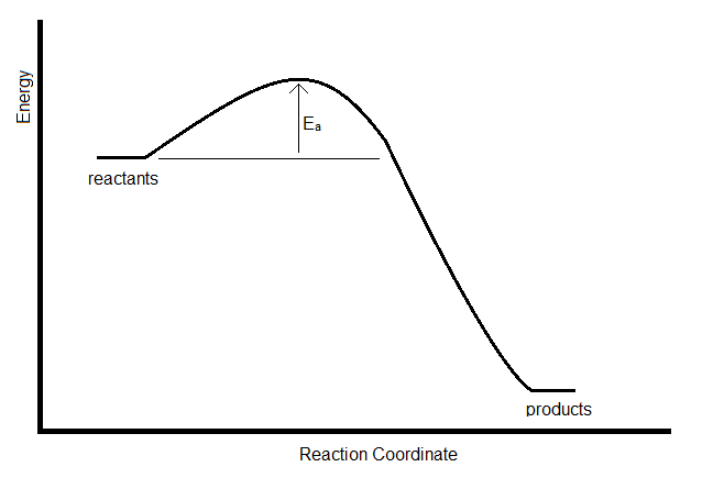
- In the equation, \(E_a\) is the activation energy
- The activation energy is the energy that must be overcome in a collision to lead to a reaction
- If the rate constant is measured at two temperatures, the activation energy can be determined by ratioing the rate constants \[ \ln \left(\frac{k_1}{k_2}\right)=\frac{E_a}{R}\left(\frac{1}{T_2}-\frac{1}{T_1}\right) \]
- If the rate constant is measured at a series of temperature, we can do a fit to find the activation energy \[ \ln (k) = -\frac{E_a}{RT} + \ln (A) \Rightarrow \ln (k) = -\frac{E_a}{R}\frac{1}{T} + \ln (A) \]
Example 11.6
For a given reaction, the rate constant doubles when the temperature is increased from \(25^\circ C\) to \(35^\circ C\). What is the Arrhenius activation energy from this reaction?
Collision Theory
- Collision theory was first introduced by Max Trautz in 1916 and William Lewis in 1918.
- The rate of a reaction in collision theory can be expressed as \[ \text{rate}=Z_{ab}F \] where \(Z_{ab}\) is the frequency of collision between A and B, and \(F\) is the fraction of those collisions that will lead to a reaction
- \(F\) has constributions from the energy of the collision and the orientation of the molecules during collision
- \(Z_{ab}\) can be taken from the kinetic molecular theory discussed previously \[ Z_{ab}=\left(\frac{8k_BT}{\pi \mu}\right)^\frac{1}{2}\sigma_{AB}[A][B] \]
The Terms in Zab
\( Z_{ab}=\left(\frac{8k_BT}{\pi \mu}\right)^\frac{1}{2}\sigma_{AB}[A][B] \)
- The first term is the average relative velocity
- \(\mu\) is the reduced mass of the A-B system
- \(\sigma_{AB}\) is the collisional cross section
- \([A]\) and \([B]\) are the concentrations of A and B
The Factor F
- \(F\) depends on activation energy and assuming Boltzmann distribution of energies \[ F=e^{-\frac{E_a}{RT}} \]
The Collision Theory Rate
- Plugging our \(F\) and \(Z_{ab}\) expressions into our rate equation \[ \text{rate}= \left(\frac{8k_BT}{\pi \mu}\right)^\frac{1}{2}\sigma_{AB} e^{-\frac{E_a}{RT}} [A][B] \]
- By comparision with the usual rate laws, \(\text{rate}=k[A][B]\) we see that \[ k = \left(\frac{8k_BT}{\pi \mu}\right)^\frac{1}{2}\sigma_{AB} e^{-\frac{E_a}{RT}} \]
- Remembering that Arrhenius found that \(k=Ae^{-\frac{E_a}{RT}}\) we see that the Arrhenius prefactor (constant) is \[ A = \left(\frac{8k_BT}{\pi \mu}\right)^\frac{1}{2}\sigma_{AB} \]
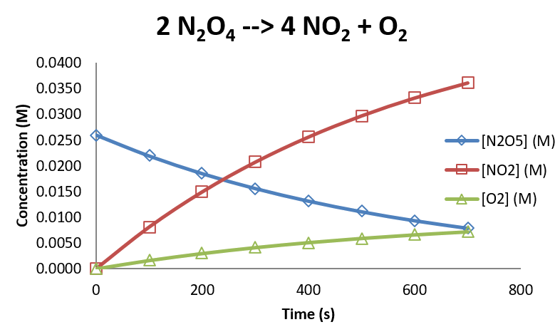
A Decomposition Example
- Consider the decomposition of \(N_2O_5\) via the reaction \(2N_2O_5 \rightarrow 4NO_2 + O_2\)
- The following data was collected under a certain set of conditions
| Time (s) | [N2O5] (M) | [NO2] (M) | [O2] (M) |
|---|---|---|---|
| 0 | 0.0260 | 0.0000 | 0.0000 |
| 100 | 0.0219 | 0.0081 | 0.0016 |
| 200 | 0.0185 | 0.0150 | 0.0030 |
| 300 | 0.0156 | 0.0207 | 0.0041 |
| 400 | 0.0132 | 0.0256 | 0.0051 |
| 500 | 0.0111 | 0.0297 | 0.0059 |
| 600 | 0.0094 | 0.0332 | 0.0066 |
| 700 | 0.0079 | 0.0361 | 0.0072 |
Our Decompostion Data Graphically
Decomposition Data Analysis
- The data for \(N_2O_5\) can be analyzed empirically to show that the reaction is first order in \(N_2O_5\), with a rate constant of \(1.697\times 10^{-3}s^{-1}\)
- The rate law for the reaction is \[ \text{rate}=1.697\times 10^{-3}s^{-1} \left[ N_2O_5 \right] \]
- The initiation of this reaction is bimolecular \[ N_2O_5 + M \leftrightharpoons N_2O_5^* + M \] where \(N_2O_5^*\) is an energetically activated form of \(N_2O_5\) which can relax into either \(N_2O_5\) or decompose to products
- Because the initiation step is bimolecular, collision theory can be used to understand the rate law
- Because the product of the bimolecular step undergoes slow conversion to product unimolecularly,the overall reaction is observed to be first order in \(N_2O_5\)
Transition State Theory
- Transition state theory ws proposed in 1935 by Henry Erying and then developed by Merrideth G. Evans and Michael Polanyi
- The theory is based on the idea that a molecular collision that leads to reaction must pass through an intermediate state known as a transition state
- For example, in the reaction \(A+BC \rightarrow AB+C\) would have an intermediate of \(ABC\) where the \(B-C\) is partially broken and the \(A-B\) bond is partially formed. \[ A+BC \rightarrow \left(A-B-C\right)^\ddagger \rightarrow AB+C \]
- This reaction is mediated by the formation of an activated complex (symbolized with the \(\ddagger\)) and the decomposition of that activated complex forms the products.
Rates in Transition State Theory
- Using the theory, the rate of a reaction can be regarded as \[ \text{rate}=\begin{multline}(\text{transition state concentration}) \\ \times (\text{decomposition frequency}) \end{multline} \]
- If the formation of the activated complex is considered to reach an equilibrium \[ K^\ddagger = \frac{[ABC]^\ddagger}{[A][BC]} \]
- So we now know that \[ [ABC]^\ddagger = K^\ddagger [A][BC] \]
- It turns out that we can write the constant as \[ K^\ddagger = e^{-\frac{\Delta G^\ddagger}{RT}} \;\; \therefore \;\; \text{rate} = (\text{frequency})[A][BC]e^{-\frac{\Delta G^\ddagger}{RT}} \]
The Frequency Term
- The frequency is taken to be equal to the vibrational frequency for the vibration of the bond being broken in the activated complex.
- This can be expressed in terms of the energy of the bond oscillations \[ E=h\nu = k_BT \;\;\text{or}\;\; \nu = \frac{k_BT}{h} \]
- So now the rate can be written as \[ \text{rate} = \frac{k_BT}{h}[A][BC]e^{-\frac{\Delta G^\ddagger}{RT}} \]
- The rate constant is now \[ k = \frac{k_BT}{h}e^{-\frac{\Delta G^\ddagger}{RT}} \]
/