Chemical Kinetics: Multi-Step Reactions
Shaun Williams, PhD
Elements of Multi-Step Reactions
Elements of Multi-Step Reactions
- Complicated reaction can be broken down into elementary steps.
- Consider the combustion of methane shown below.
Reversible Steps
- When we consider an elementary reaction, we often ignore the reverse reaction. $$ \begin{align} \mathrm{A} & \xrightarrow{k_1} \mathrm{B} \\ \mathrm{B} & \xrightarrow{k_{-1}} \mathrm{A} \end{align} $$
- If the reverse reaction is extremely slow, it could be ignored
- Usually, we must include the reverse steps in out analysis.
- We're going to first analyze the simplest case, a reversible unimolecular reaction $$ \mathrm{A} \xrightleftharpoons{k_1}{k_{-1}} \mathrm{B} $$
Reversible Unimolecular Elementary Reaction
$$ \mathrm{A} \xrightleftharpoons{k_1}{k_{-1}} \mathrm{B} $$
- Let write the rate law for this reaction $$ \begin{align} \frac{d\conc{A}}{dt} & = -k_1 \conc{A} + k_{-1}\conc{B} \\ \frac{d\conc{B}}{dt} & = k_1 \conc{A} - k_{-1}\conc{B} \end{align} $$
- Give initial concentrations of \( \conc{A}_0 \) and \( \conc{B}_0 \) we can define the extent of the reaction, \( x \) $$ x = \conc{B} - \conc{B}_0 = \conc{A}_0 - \conc{A} $$ note that the initial concentrations are constant.
Developing the Integrated Rate Law
- We need to use our rate law to develope an integrated rate law
$$ \begin{align} v & = \frac{d\conc{B}}{dt} = -\frac{d\conc{A}}{dt} = \frac{dx}{dt} \\ & = k_1 \conc{A} - k_{-1}\conc{B} = k_1 \left( \conc{A}_0 - x \right) - k_{-1}\left( \conc{B}_0 + x \right) = \frac{dx}{dt} \\ dt & = \frac{dx}{k_1 \left( \conc{A}_0 - x \right) - k_{-1}\left( \conc{B}_0 + x \right)} \\ & = \frac{dx}{k_1 \conc{A}_0 -k_1 x - k_{-1}\conc{B}_0 - k_{-1}x} \\ & = \frac{dx}{k_1 \conc{A}_0 - k_{-1}\conc{B}_0 - \left( k_1 + k_{-1} \right) x} \end{align} $$
Continuing
$$ dt = \frac{dx}{k_1 \conc{A}_0 - k_{-1}\conc{B}_0 - \left( k_1 + k_{-1} \right) x} $$
$$ \begin{align} dt & = \frac{dx}{\left( k_1 + k_{-1} \right) \left( \frac{k_1}{k_1 + k_{-1}} \conc{A}_0 - \frac{k_{-1}}{k_1 + k_{-1}}\conc{B}_0 - x \right)} \\ -\left( k_1 + k_{-1} \right)\, dt & = \frac{dx}{\frac{k_{-1}}{k_1 + k_{-1}}\conc{B}_0 - \frac{k_1}{k_1 + k_{-1}} \conc{A}_0 + x} \\ -\left( k_1 + k_{-1} \right)\, dt & = \frac{dx}{\left(\frac{1}{k_1 + k_{-1}}\right)\left( k_{-1}\conc{B}_0 - k_1\conc{A}_0\right) + x } \\ \end{align} $$
Almost there...
$$ -\left( k_1 + k_{-1} \right)\, dt = \frac{dx}{\left(\frac{1}{k_1 + k_{-1}}\right)\left( k_{-1}\conc{B}_0 - k_1\conc{A}_0\right) + x } $$
$$ \begin{align} \int_0^t -\left( k_1 + k_{-1} \right)\, dt & = \int_0^x \frac{dx'}{\left(\frac{1}{k_1 + k_{-1}}\right)\left( k_{-1}\conc{B}_0 - k_1\conc{A}_0\right) + x' } \\ -\left( k_1 + k_{-1} \right) t & = \ln \left[ \frac{\left(\frac{1}{k_1 + k_{-1}}\right)\left( k_{-1}\conc{B}_0 - k_1\conc{A}_0\right) + x}{\left(\frac{1}{k_1 + k_{-1}}\right)\left( k_{-1}\conc{B}_0 - k_1\conc{A}_0\right)} \right] \\ x & = \left( \frac{k_1\conc{A}_0 - k_{-1}\conc{B}_0}{k_1 + k_{-1}} \right) \left( 1 - e^{-\left( k_1 + k_{-1} \right)t} \right) \end{align} $$
Finally, the Integrated Rate Law
$$ x = \left( \frac{k_1\conc{A}_0 - k_{-1}\conc{B}_0}{k_1 + k_{-1}} \right) \left( 1 - e^{-\left( k_1 + k_{-1} \right)t} \right) $$
$$ \begin{align} \conc{A} & = \conc{A}_0 - x = \conc{A}_0 - \left( \frac{k_1\conc{A}_0 - k_{-1}\conc{B}_0}{k_1 + k_{-1}} \right) \left( 1 - e^{-\left( k_1 + k_{-1} \right)t} \right) \\ \conc{B} & = \conc{B}_0 + x = \conc{B}_0 + \left( \frac{k_1\conc{A}_0 - k_{-1}\conc{B}_0}{k_1 + k_{-1}} \right) \left( 1 - e^{-\left( k_1 + k_{-1} \right)t} \right) \end{align} $$ Note that $$ \begin{align} \lim_{k_{-1}\rightarrow 0} \conc{A} & = \conc{A}_0 - \left( \frac{k_1\conc{A}_0}{k_1} \right) \left( 1 - e^{-k_1 t} \right) \\ \lim_{k_{-1}\rightarrow 0} \conc{A} & = \conc{A}_0 - \left( \conc{A}_0 - \conc{A}_0 e^{-k_1 t} \right) = \conc{A}_0e^{-k_1 t} \end{align} $$
Equilibrium
- At equilibrium the rate is zero so we would have $$ -\frac{d\conc{A}}{dt} = \frac{d\conc{B}}{dt} = k_1 \conc{A}_{eq} - k_{-1} \conc{B}_{eq} = 0 $$
- Doing some quick math we find that $$ K_{eq} =\frac{\conc{B}_{eq}}{\conc{A}_{eq}} = \frac{k_1}{k_{-1}} $$
Parallel Reactions
- Competing (parallel) reactions draw from the same reactant(s) to form different products $$ \chem{A \xrightarrow{k_1} B},\; \chem{A \xrightarrow{k_2} C} $$
- The overall reaction velocity will be $$ v = -\frac{d\conc{A}}{dt} = k_1 \conc{A} + k_2 \conc{A} = \left( k_1 + k_2 \right) \conc{A} $$
- Using the same method we have used several times now, we can generate the corresponding integrated rate law $$ \conc{A}=\conc{A}_0e^{-\left( k_1 + k_2 \right)t} $$
The Products in Parallel Reactions
$$ \conc{A}=\conc{A}_0e^{-\left( k_1 + k_2 \right)t} $$
- We can use this integrate rate law to analyze the products.
- First \( \chem{B} \) $$ \begin{align} \frac{d\conc{B}}{dt} & = k_1 \conc{A} = k_1 \conc{A}_0e^{-\left( k_1 + k_2 \right)t} \\ \conc{B} & = \frac{k_1 \conc{A}_0}{k_1+k_2}\left[ 1-e^{-\left( k_1 + k_2 \right)t} \right] \end{align} $$
- Similarly $$ \conc{C} = \frac{k_2 \conc{A}_0}{k_1+k_2}\left[ 1-e^{-\left( k_1 + k_2 \right)t} \right] $$
- Therefore \( \frac{\conc{B}}{\conc{C}} = \frac{k_1}{k_2} \)
Example 14.1
The compound \(\beta\)-pinene isomerizes at 650 K to either 4-isopropenyl-1-methylcyclohexene (call it IMC), with a rate constant of \( k_1 = 0.22\,\mathrm{s}^{-1} \), or to myrcene, with a rate constant of \( k_2 = 0.13\,\mathrm{s}^{-1} \). If the reaction is carried out under kinetic control, what is the ratio of IMC to myrcene, and what is the half-life of the \(\beta\)-pinene?
Sequential Reactions
- Sequential reactions are the basis of multi-step reactions
- Products made in one step can be used in these next
- There are chemical intermediates
- The simplest set of sequential reactions is $$ \chem{A} \xrightarrow{k_1} \chem{B} \xrightarrow{k_2} \chem{C} $$
- Let's start by assuming that \( \conc{A}_0\ne 0 \) and \( \conc{B}_0 = \conc{C}_0 = 0 \)
- So, for \(\chem{A}\) it is easy $$ -\frac{d\conc{A}}{dt}=k_1\conc{A}\;\;\;\mathrm{and}\;\;\;\conc{A}=\conc{A}_0 e^{-k_1 t} $$
- The other compounds are more difficult.
Finding B
$$ \begin{align} \frac{d\conc{B}}{dt} & = k_1 \conc{A} - k_2 \conc{B} \\ & = k_1 \conc{A}_0 e^{-k_1 t} - k_2 \conc{B} \end{align} $$
- It is not the purpose of this class to drag you through the relatively difficult task of solving the differential equation. It is in your book on page 484 if you are interested.
- The result is that $$ \conc{B} = \frac{\conc{A}_0k_1}{k_2-k_1}\left( e^{-k_1t}-e^{-k_2t} \right) $$
Finding C
$$ \begin{align} \conc{A} & =\conc{A}_0 e^{-k_1 t} \\ \conc{B} & = \frac{\conc{A}_0k_1}{k_2-k_1}\left( e^{-k_1t}-e^{-k_2t} \right) \end{align} $$
- We can find an expression for C by substitution $$ \begin{align} \conc{C} & = \conc{A}_0 -\conc{A}-\conc{B} \\ & = \conc{A}_0 - \conc{A}_0 e^{-k_1 t} - \frac{\conc{A}_0k_1}{k_2-k_1}\left( e^{-k_1t}-e^{-k_2t} \right) \\ & = \conc{A}_0\left( 1 - \frac{k_2 e^{-k_1t}-k_1e^{-k_2t}}{k_2-k_1} \right) \end{align} $$
Approximations in Kinetics
Approximations in Kinetics
- There are times when thetechniques we have already developed work fine.
- Sometime, however, the multi-step reaction is too complicated to get an analytical solution $$ \begin{align} \chem{A+B} & \xrightleftharpoons{k_1}{k_{-1}} \chem{C} \xrightarrow{k_2} \chem{D} \\ \frac{d\conc{A}}{dt} & = -k_1 \conc{A}\conc{B} + k_{-1}\conc{C} \\ \frac{d\conc{C}}{dt} & = k_1\conc{A}\conc{B} - k_{-1}\conc{C}-k_2\conc{C} \\ \frac{d\conc{D}}{dt} & = k_2 \conc{C} \end{align} $$
- We still need a solution so we need to develope approximation methods
The Steady-State Approximation
- The intermediates in a series of elementary reactions are often extremely reaction
- As such, the react away much faster than they are created
- This results in the concentration of the intermediates hitting equilibrium very quickly
- When this set of conditions exist, the steady-state approximation is useful
- The steady state approximations assumes that the concentration of intermediates change so slowly that they can be treated as constant over short times
Using the Steady-State Approximation
$$ \chem{A+B} \xrightleftharpoons{k_1}{k_{-1}} \chem{C} \xrightarrow{k_2} \chem{D} $$
- Looking at our intermdiate $$ \frac{d\conc{C}}{dt} = k_1\conc{A}\conc{B} - k_{-1}\conc{C}-k_2\conc{C} $$
- Applying the Steady-State Approximation $$ \frac{d\conc{C}}{dt} = 0 = k_1\conc{A}\conc{B} - k_{-1}\conc{C}_{SS}-k_2\conc{C}_{SS} $$
- Solving for \(\conc{C}_{SS}\) we get $$ \conc{C}_{SS}=\frac{k_1\conc{A}\conc{B}}{k_{-1}+k_2} $$
The Steady-State Approximation Effect on other Species
- Let's look at \(\chem{A}\) under this assumption (note the ' indicates that it is approximate) $$ \begin{align} \frac{d\conc{A}'}{dt} & = -k_1 \conc{A}'\conc{B}' + k_{-1}\conc{C}_{SS} \\ & = -k_1 \conc{A}'\conc{B}' + k_{-1}\frac{k_1\conc{A}'\conc{B}'}{k_{-1}+k_2} \\ & = \left( -1+\frac{k_{-1}}{k_{-1}+k_2} \right) k_1 \conc{A}'\conc{B}' \\ -\frac{d\conc{A}'}{dt} & = \left( 1-\frac{k_{-1}}{k_{-1}+k_2} \right) k_1 \conc{A}'\conc{B}' \end{align} $$
- As long as \(\chem{A}\) and \(\chem{B}\) react at the same rate: \(\conc{B}_0-\conc{B}'=\conc{A}_0-\conc{A}'\)
Continuing the Analysis of \(\chem{A}\)
$$ \begin{align} -\frac{d\conc{A}'}{dt} & = \left( 1-\frac{k_{-1}}{k_{-1}+k_2} \right) k_1 \conc{A}'\conc{B}' \\ \conc{B}_0-\conc{B}' & =\conc{A}_0-\conc{A}' \end{align} $$
- Using these together we can find that $$ -\frac{d\conc{A}'}{dt} = \left( 1-\frac{k_{-1}}{k_{-1}+k_2} \right) k_1 \conc{A}'\left( \conc{B}_0 - \conc{A}_0 + \conc{A}' \right) $$
- Isolating terms $$ -\frac{d\conc{A}'}{\conc{A}'\left( \conc{B}_0 - \conc{A}_0 + \conc{A}' \right)} = \left( 1 - \frac{k_{-1}}{k_{-1}+k_2} \right) k_1\,dt $$
Finishing the Analysis of \(\chem{A}\)
$$ -\frac{d\conc{A}'}{\conc{A}'\left( \conc{B}_0 - \conc{A}_0 + \conc{A}' \right)} = \left( 1 - \frac{k_{-1}}{k_{-1}+k_2} \right) k_1\,dt $$
- Integrating this we arrive at $$ \begin{align} \frac{1}{\conc{B}_0-\conc{A}_0} & \left[ \ln \left( \frac{\conc{B}_0-\conc{A}_0+\conc{A}'}{\conc{A}'}-\ln \left( \frac{\conc{B}_0}{\conc{A}_0} \right) \right) \right] \\ & = k_1 \left( 1-\frac{k_{-1}}{k_{-1}+k_2} \right) t \end{align} $$
- Doing a lot of algebra we find that $$ \begin{multline} \conc{A}' = \conc{A}_0 \left( 1-\frac{\conc{A}_0}{\conc{B}_0} \right) \\ \left\{ \exp \left[ \left( \conc{B}_0 - \conc{A}_0 \right) \left( 1-\frac{k_{-1}}{k_{-1}+k_2} \right)k_1 t \right] - \frac{\conc{A}_0}{\conc{B}_0} \right\}^{-1} \end{multline} $$
Example 14.2
Show that the last equation correctly predicts the rate law of an irreversible bimolecular reaction \( \chem{A+B} \xrightarrow{k_1} \chem{D} \) in the limit that \( k_{-1} \ll k_1 \)
The Fast-Equilibrium Approximation
$$ \chem{A+B} \xrightleftharpoons{k_1}{k_{-1}} \chem{C} \xrightarrow{k_2} \chem{D} $$
- If \( k_{-1} \gg k_2 \) then the fast-equilibrium approximation may be applicable.
- Due to the relative sizes of the rate constants, A, B, and C quickly reach their equilibrium values. $$ \frac{\conc{C}}{\conc{A}{\conc{B}}} \approx K_1 = \frac{k_1}{k_{-1}} $$
- Solving this we find that $$ \conc{C}_{fe} = \frac{k_1}{k_{-1}}\conc{A}\conc{B} $$
The Initial Rate Approximation
- We can estimate the value of a derivative by numerical differentiation $$ \frac{d\conc{A}}{dt} \approx \frac{\conc{A}_{t+\delta t}-\conc{A}_t}{\delta t} $$
- Therefore, we can measure the concentrations very soon after starting the reaction and solve for the rate law without having to do calculus
- If a reaction has two reactants A and B then all we know is that $$ -\frac{d\conc{A}}{dt} = k\conc{A}^n\conc{B}^m $$ \(n \) and \(m \) can be non-integers for complex reactions
Experiment
To find the initial rate, we run three experiments
- The initial concentrations are each \( 1.0\,\mathrm{mol}\,\mathrm{L}^{-1} \). The concentration of A drops to \( 0.90\,\mathrm{mol}\,\mathrm{L}^{-1} \) at 22.4 seconds after starting the reaction.
- We double the initial concentration of B to \( 2.0\,\mathrm{mol}\,\mathrm{L}^{-1} \) and now find that A reaches \( 0.90\,\mathrm{mol}\,\mathrm{L}^{-1} \) at 11.1 seconds.
- We double the initial concentration of A to \( 2.0\,\mathrm{mol}\,\mathrm{L}^{-1} \), (with B back at \( 1.0\,\mathrm{mol}\,\mathrm{L}^{-1} \)) and find that A reaches \( 1.90\,\mathrm{mol}\,\mathrm{L}^{-1} \) at 5.3 seconds.
We are going to replace \( d\conc{A} \) in the rate law by the in concentration of A.
Solving the Experiment
$$ \begin{align} -\frac{d\conc{A}}{dt} = & k\conc{A}^n\conc{B}^m \\ -\frac{\Delta \conc{A}}{\Delta t} \approx & k\conc{A}_0^n\conc{B}_0^m \\ \frac{0.10}{22.4} \approx & k\left( 1.0 \right)^n \left( 1.0 \right)^m \\ \frac{0.10}{11.1} \approx & k\left( 1.0 \right)^n \left( 2.0 \right)^m \\ \frac{0.10}{5.3} \approx & k\left( 2.0 \right)^n \left( 1.0 \right)^m \\ \end{align} $$ Dividing the first equation into the second and third we find that $$ 2\approx \left(2.0\right)^m \;\;\; 4 \approx \left(2.0\right)^n $$ Thus \(m=1\) and \(n=2\).
Solving the Experiment Continued
- Our rate law has become $$ -\frac{d\conc{A}}{dt}=k\conc{A}^2 \conc{B} $$
- We can now estimate the rate constant: $$ k=\frac{0.10\,\mathrm{mol}\,\mathrm{L}^{-1}}{22.4\,\mathrm{s}\left( 1.0\,\mathrm{mol}\,\mathrm{L}^{-1} \right)^3}=0.0045\,\mathrm{L}^2\,\mathrm{mol}^{-2}\,\mathrm{s}^{-1} $$
The Pseudo-Lower Order Approximation
$$ \chem{A+B} \xrightleftharpoons{k_1}{k_{-1}} \chem{C} \xrightarrow{k_2} \chem{D} $$
- Carry out the reaction with a huge concentration of B
- Having an large excess of one reactant makes that reactants concentration effectively constant at \(\conc{B}_0\)
- The reaction velocity is, therefore $$ \frac{d\conc{C}}{dt}\approx k_1\conc{A}\conc{B}_0 - \left( k_{-1}+k_2 \right) \conc{C} $$
- The steady-state concentration of C can be solved directly $$ \conc{C}_{(1)} = \frac{k_1\conc{A}\conc{B}_0}{k_{-1}+k_2} $$
Chain Reactions
Chain Reactions
- A chain reaction is a self-propagating reaction series consisting ofr four categories of reactions
$$ \begin{align} \mathrm{initiation:} & \chem{H_2\rightarrow 2H} \\ & \chem{O_2 \rightarrow 2O} \\ \mathrm{branching:} & \chem{H + O_2 \rightarrow OH + O} \\ & \chem{O+H_2\rightarrow OH+H} \\ \mathrm{propagation:} & \chem{OH+H_2\rightarrow H_2O +H} \\ \mathrm{termination:} & \chem{2H+M\rightarrow H_2+M} \\ & \chem{H+O_2+M\rightarrow HO_2+M} \\ & \chem{HO_2 + OH \rightarrow H_2O + O_2} \\ & \chem{HO_2+H\rightarrow H_2+O_2} \end{align} $$
- The chain reaction is only effective at self-propagation when the kinetic chain length (\(v_\mathrm{propagation}:v_\mathrm{initiation}\)) is large
Reaction Networks
The Atmosphere
Different gas densities and distances from the earth's surface favor different heating and cooling mechanisms
- Troposhere (0 to ~18 km above the earth's surface)
- \(T\) decreases with altitude.
- The atmosphere is largely transparent to the visible and infrared
- This level of the atmosphere is heated partly by convention and partly by infrared radiation
- Molecules that absorb the infrared are most abundant in this region of the atmosphere
The Atmosphere Continued
- Stratosphere (~18 to ~50 km)
- \(T\) increases with altitude
- This layer is heated by chemical reactions
- The formation and destruction of \(\chem{O_3}\) contributes to the heating of this region
- These reactions are initiated by the sun's ultraviolet radiation
- Because of the need for solar radiation, this mechanism increases as altitude increases
More About The Atmosphere
- Mesosphere (~50 to ~90 km)
- \(T\) decreases with altitude
- Gas densities have dropped so reactions slow down
- Additional cooling by infrared radiation of thermally excited \(\chem{CO_2}\) into the infrared transparent upper atmosphere
- In this region, the atmosphere reaches its coldest temperatures, as low as 100 K under extreme conditions.
Top of the Atmosphere
- Thermosphere (~90 to ~500-1000 km)
- \(T\) increases with altitude
- This region is heated by the direct photodissociation and photoionization of \(\chem{O_2}\) and \(\chem{N_2}\)
- These endothermic processes convert high-frequency ultraviolet light into kinetic energy of separated atoms and atomic ions
- This results is temperatures on the order of 1000 K.
- The ions in the lower sections interact most strongly with ground-based radio transmissions so it is also known as the ionosphere
The Chapman Mechanism
- The Chapman Mechanism is a model for the atmospheric \(\chem{O_3}\) cycle
- At the temperatures and radiation intensity at about 30 km $$ \begin{align} & \chem{O_2} + \mathrm{h}\nu \xrightarrow{j_1} \chem{2O} & j_1 &= 5.2\times 10^{-11}\,\mathrm{s}^{-1} \\ & \chem{O + O_2 + M} \xrightarrow{k_2} \chem{O_3+M} & k_2 &= 5.6\times 10^{-34}\,\mathrm{cm}^{6}\,\mathrm{mol}^{-2}\,\mathrm{s}^{-1} \\ & \chem{O_3} + \mathrm{h}\nu \xrightarrow{j_3} \chem{O+O_2} & j_3 &= 9.5\times 10^{-4}\,\mathrm{s}^{-1} \\ & \chem{O+O_3} \xrightarrow{k_4} \chem{2O_2} & k_4 &= 1.0\times 10^{-15}\,\mathrm{cm}^{3}\,\mathrm{mol}^{-1}\,\mathrm{s}^{-1} \end{align} $$
First Analysis
- We can apply the steady-state approximation to all the compounds since they are all intermediates $$ \begin{align} \frac{d\conc{O}}{dt} &= 2j_1\conc{O_2}-k_2\conc{O}\conc{O_2}\conc{M}+j_3\conc{O_3}-k_4\conc{O}\conc{O_3} \\ &= 0 \\ \frac{d\conc{O_2}}{dt} &= -j_1\conc{O_2}-k_2\conc{O}\conc{O_2}\conc{M}+j_3\conc{O_3}+2k_4\conc{O}\conc{O_3} \\ &= 0 \\ \frac{d\conc{O_3}}{dt} &= k_2\conc{O}\conc{O_2}\conc{M}-j_3\conc{O_3}-k_4\conc{O}\conc{O_3} \\ &= 0 \end{align} $$
- The abundance of \(\chem{N_2}\) is not affected by this series of reaction so we can assume that \(\conc{M}\) is constant, \(\conc{M}\approx 6.7\times 10^{17}\,\mathrm{cm}^{-3} = 1.1\times 10^{-6}\,\mathrm{mol}\,\mathrm{cm}^{-3}\)
First Analysis Continued
- Adding the second and third of the rate equations together we find $$ -j_1\conc{O_2}+k_4\conc{O}\conc{O_3}=0 $$
- We can solve this for \(\conc{O}\) $$ \conc{O}=\frac{j_1\conc{O_2}}{k_4\conc{O_3}} $$
- Using this with the first rate equation $$ \begin{align} \conc{O_3} &= \frac{1}{j_3-k_4\conc{O}}\left( k_2\conc{O}\conc{O_2}\conc{M} - 2j_1\conc{O_2} \right) \\ &= \frac{1}{j_3-\left( \frac{j_1\conc{O_2}}{\conc{O_3}} \right)} \left( \frac{k_2j_1\conc{O_2}^2\conc{M}}{k_4\conc{O_3}}-2j_1\conc{O_2} \right) \end{align} $$
First Analysis Concluded
- We can multiply through by \(\conc{O_3}\) to remove it from the denominators
- This allows us to find that $$ \conc{O_3}=1.8\times 10^{13}\,\mathrm{cm}^{-3} $$
- This can be used to find that $$ \conc{O}=3.6\times 10^{8}\,\mathrm{cm}^{-3} $$
- The actual \(\chem{O_3}\) density is lower by a factor of 2 to 4 due to nitrogen, hydrogen, and chlorine cycles that also participate
The \(\chem{HO_x}\) Cycle
The \(\chem{HO_x}\) cycle is dominated by two systems
- Below an altitude of 30 km $$ \begin{align} \chem{OH+O_3} &\rightarrow \chem{HO_2+O_2} \\ \chem{HO_2+O_3} &\rightarrow \chem{OH+O_2+O_2} \end{align} $$ $$\mathrm{Net:}\;\chem{2O_3\rightarrow 3O_2} $$
- Above an altitude of 40 km $$ \begin{align} \chem{OH+O} &\rightarrow \chem{H+O_1} \\ \chem{H+O_2+M} &\rightarrow \chem{HO_2+M} \\ \chem{HO_2+O} &\rightarrow \chem{OH+O_2} \end{align} $$ $$\mathrm{Net:}\;\chem{2O\rightarrow O_2} $$
The \(\chem{NO_x}\) Cycle
$$ \begin{align} \chem{NO+O_3} &\rightarrow \chem{NO_2+O_2} \\ \chem{NO_2+O} &\rightarrow \chem{NO+O_2} \\ \chem{NO_2+OH+M} &\rightarrow \chem{HNO_3+M} \end{align} $$ $$ \mathrm{Net:}\;\chem{O_3+O+NO_2+OH\rightarrow 2O_2+HNO_3} $$
The \(\chem{ClO_x}\) Cycle
$$ \begin{align} \chem{CCl_2F_2}+h\nu &\rightarrow \chem{CF_2Cl+Cl} \\ \chem{Cl+O_3} &\rightarrow \chem{ClO+O_2} \\ \chem{ClO+O} &\rightarrow \chem{Cl+O_2} \\ \chem{Cl+CH_4} &\rightarrow \chem{HCl+CH_3} \end{align} $$ $$ \mathrm{Net}\;\chem{CCl_2F_2+O_3+O+CH_4}+h\nu \rightarrow \chem{2O_2+CF_2Cl+HCl+CH_3} $$
Example 14.3
Use the concentration of atomic oxygen and ozone as determined by the Chapman mechanism to find an expression for the steady-state concentration of \(\chem{NO}\), which appears as an intermediate in the \(\chem{NO_x}\) cycle, in terms of \(\conc{NO_2}\), \(\conc{O_2}\), \(\conc{O_3}\), and relevant rate constants. Assume for simplicity that no other reactions contribute significantly to the \(\chem{NO}\) concentrations.
Enzyme Catalysis
- Enzymes are macromolecules that catalyze biochemical reactions
- The often increase reaction rate by over eight orders of magnitude
- Most enzymes are made up over 1000 atoms
- Enzymes may be pure proteins or part protein (the apoenzyme) and part non-protein (the coenzyme)
- In many cases, enzymes are much larger than the principal reactants, called substrates
- Like all catalysts, the reactants form a complex with the catalyst and in this complex they react more quickly
Central Questions of Enzyme-Substrate Systems
- How can we describe the structure of molecules with so many stable conformers?
- How does this structure influence the enzyme's biochemical function?
- What are the thermodynamics and kinetics governing the enzyme's biochemical function?
Biomolecular Structure
- Typically to understand structure we would use infrared spectroscopy and microwave spectroscopy
- Very large molecules rarely have a single geometry
- As such, their vibrational spectrum is nearly a continuous series of absorptions throughout the entire range, \(<3000\, \mathrm{cm}^{-1}\)
- Biomolecules are often found in water which has very strong IR absorptions
- So how do we analyze their structure
- electronic spectroscopy
- NMR spectroscopy
- optical rotation studies
- x-ray diffraction of crystalized or fibrous biochemicals
Electronic Spectroscopy of Biomolecules
- The spectroscopy of electronic transitions is most easily carried out on those molecules with relatively low-lying excited states.
- Usually, ultraviolet and visible wavelength spectroscopy of biomolecules is usually sensitive to those regions of the molecule with a metal or sulfur atom, or by some other aromatic functional group
- These sites on molecules are called chromophores
- Chromophores offer the opportunity to probe large macromolecules at a specific location
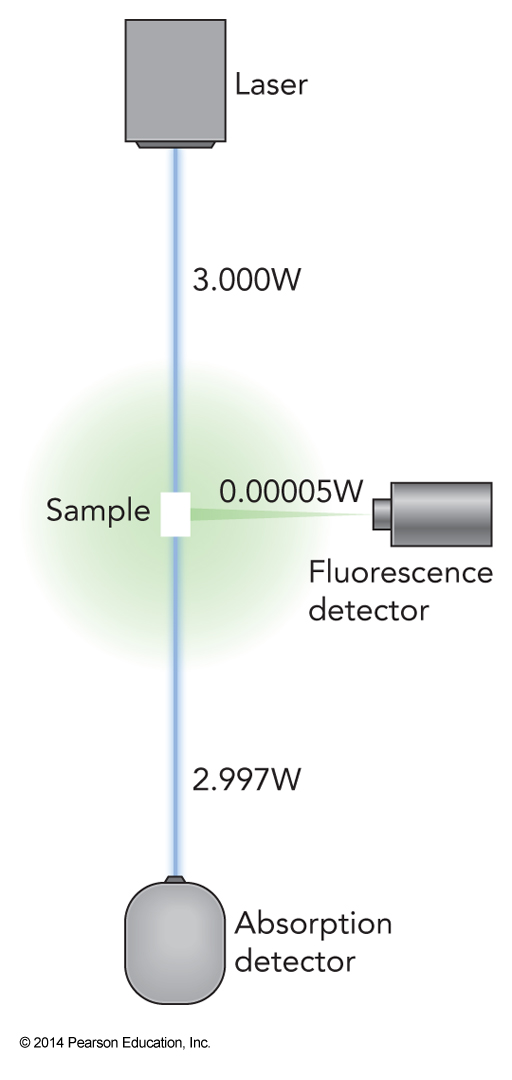
- It is more common to measure emitted fluorescence from chromophores than measuring absorption
Spectroscopy of Protein Sample
Enzyme Kinetics: The Michaelis-Menton Equation
$$ \chem{E+S} \xrightleftharpoons{k_1}{k_{-1}} \chem{ES} \xrightleftharpoons{k_2}{k_{-2}} \chem{EP} \xrightleftharpoons{k_3}{k_{-3}} \chem{E+P} $$
- Enzyme concentration is less that 1% the substrate concentrations so \(\chem{ES}\) is essentially a steady state
- The third step is extremely fast compared the first and second so we can treat this as a two step mechanism $$ \chem{E+S} \xrightleftharpoons{k_1}{k_{-1}} \chem{ES} \xrightleftharpoons{k_2}{k_{-2}} \chem{E+P} $$
- If we focus on the early reaction, \(\conc{P}\) is small so the second step is essentially irreversible $$ \chem{E+S} \xrightleftharpoons{k_1}{k_{-1}} \chem{ES} \xrightarrow{k_2} \chem{E+P} $$
Starting Work on the Rate Law
$$ \chem{E+S} \xrightleftharpoons{k_1}{k_{-1}} \chem{ES} \xrightarrow{k_2} \chem{E+P} $$ $$ \begin{align} \frac{d\conc{P}}{dt} &= k_2\conc{ES} \\ \frac{d\conc{ES}}{dt} &= k_1\conc{E}\conc{S}-k_{-1}\conc{ES}-k_2\conc{ES} \\ &= k_1\conc{E}\conc{S}-k_{-1}\conc{ES}_{ss}-k_2\conc{ES}_{ss}\overset{ss}{=}0 \\ \conc{ES}_{ss} &= \frac{k_1\conc{E}\conc{S}}{k_{-1}+k_2} = \frac{k_1}{k_{-1}+k_2}\conc{E}\conc{S} \end{align} $$ We can simplify this equation by defining the Michaelis-Menton constant, \( K_M\equiv \frac{k_{-1}+k_2}{k_1} \), therefore \( \conc{ES}_{ss} = \frac{\conc{E}\conc{S}}{K_M} \)
More Work on the Rate Law
$$ \chem{E+S} \xrightleftharpoons{k_1}{k_{-1}} \chem{ES} \xrightarrow{k_2} \chem{E+P} $$ $$ \begin{align} \conc{ES}_{ss} &= \frac{\conc{E}\conc{S}}{K_M} \\ \conc{E}_0 &= \conc{E}+\conc{ES} \\ \conc{ES}_{ss} &= \frac{\left( \conc{E}_0-\conc{ES}_{ss} \right)\conc{S}}{K_M} \\ &= \frac{\conc{E}_0\conc{S}}{K_M}-\frac{\conc{ES}_{ss}\conc{S}}{K_M} \\ \conc{ES}_{ss}\left( 1+\frac{\conc{S}}{K_M} \right) &= \frac{\conc{E}_0\conc{S}}{K_M} \\ \conc{ES}_{ss} &= \frac{\bfrac{\conc{E}_0\conc{S}}{K_M}}{\bfrac{1+\conc{S}}{K_M}} = \frac{\conc{E}_0\conc{S}}{K_M+\conc{S}} \end{align} $$
Continuing Work on the Rate Law
$$ \chem{E+S} \xrightleftharpoons{k_1}{k_{-1}} \chem{ES} \xrightarrow{k_2} \chem{E+P} $$ $$ \frac{d\conc{P}}{dt} = k_2\conc{ES} $$ $$ \conc{ES}_{ss} = \frac{\conc{E}_0\conc{S}}{K_M+\conc{S}} $$ Combining the last two equatons we find that $$ \frac{d\conc{P}}{dt} = k_2\conc{ES}_{ss} = k_2 \frac{\conc{E}_0\conc{S}}{K_M+\conc{S}} $$ This is one form of the Michaelis-Menton equation. All the values on the right-hand side (RHS) are constant except for \(\conc{S}\).
Analysis of the Michaelis-Menton Equation
$$ \frac{d\conc{P}}{dt} = k_2 \frac{\conc{E}_0\conc{S}}{K_M+\conc{S}} $$
- Let's look at two limits of the Michaelis-Menton equation.
- Let's look at the low limit $$ \lim_{\conc{S}\rightarrow 0} \frac{d\conc{P}}{dt} = \frac{k_2\conc{E}_0\conc{S}}{K_M} $$
- Let's look at the high limit $$ \lim_{\conc{S}\rightarrow \infty} \frac{d\conc{P}}{dt} = \frac{k_2\conc{E}_0\conc{S}}{\conc{S}} = k_2\conc{E}_0 $$
Modification of the Michaelis-Menton Equation
- Considering the high limit on \(\conc{S}\) we can define the maximum velocity $$ v_{max}=k_2 \conc{E}_0 $$
- Using this equation we can modify the Michaelis-Menton equation $$ \frac{d\conc{P}}{dt} = k_2 \frac{\conc{E}_0\conc{S}}{K_M+\conc{S}} = k_2 \conc{E}_0 \frac{\conc{S}}{K_M+\conc{S}} = v_{max} \frac{\conc{S}}{K_M+\conc{S}} $$
- Note that the rate constant \(k_2\) is also known as the enzymatic turnover number
- the number of substrate molecules converted to product per unit time
- it is often written as \(k_{cat}\)
The Michaelis-Menton Reaction Velocity
![The predicted reaction velocity d[P]/dt for early times in an enzyme-catalyzed reaction is graphed as a function of substrate concentration [S]. The plot show the rise toward the v-max limit.](./figures/Chapter 14/14_05_Figure.jpg)
Uses of Michaelis-Menton Equation
- The fraction of occupied reactive sites can be calculated from \(K_M\) $$ f_{ES}=\frac{\conc{ES}}{\conc{E}_0}=\frac{\conc{S}}{\conc{S}+K_M} $$
- One common way of finding \(K_M\) is from a Lineweaver-Burk plot which is based on $$ \frac{1}{\bfrac{d\conc{P}}{dt}} = \frac{1}{v_{max}} + \frac{K_M}{v_{max}\conc{S}} $$
Complication
- A complication may arise when an inhibitor is present
- Inhibitor is a substance that blocks the catalytic activity of the enzyme
- In the simpliest case, the inhibitor binds at the same enzyme site that the substrate uses
- This binding can be written as $$ \chem{E+I}\xrightleftharpoons{k_3}{k_{-3}} \chem{EI} $$ with an equilibrium constant of $$ K_3=\frac{k_3}{k_{-3}}=\frac{\conc{EI}}{\conc{E}\conc{I}} $$
Applying the Complication
- Applying our inhibitor equations to our enzyme concentrations we find that $$ \begin{align} \conc{E}_0 &= \conc{E}+\conc{ES}+\conc{EI}=\conc{E}+\conc{ES}+K_3\conc{E}\conc{I} \\ \conc{E} &= \frac{\conc{E}_0-\conc{ES}}{1+K_3\conc{I}} \end{align} $$
- Applying this change to \(\conc{ES}_{ss}\) $$ \conc{ES}_{ss} = \frac{\conc{E}\conc{S}}{K_M} = \frac{\left( \conc{E}_0 - \conc{ES}_{ss} \right) \conc{S}}{K_M \left( 1+K_3\conc{I} \right)} $$ Doing a lot of algebra we can arrive at $$ \conc{ES}_{ss} = \frac{\conc{E}_0\conc{S}}{K_M+K_MK_3\conc{I}+\conc{S}} $$
The Inhibited Michaelis-Menton Equation
- Applying our inhibited steady-state concentration to our production rate we arrive at $$ \frac{d\conc{P}}{dt} = \frac{k_2\conc{E}_0\conc{S}}{K_M+K_MK_3\conc{I}+\conc{S}} $$
More Enzyme Information
- The location on the enzyme surface where the substrate binds is called the active site
- The ratio of the number of active sites occupied to the total number of available active site is called the coverage, \(\theta\) $$ \begin{align} \theta &= \frac{\conc{ES}}{\conc{E}_0} = \frac{k_1\conc{S}}{k_{-1}+k_2+k_1\conc{S}} \\ &= \frac{\left( \frac{k_1}{k_{-1}+k_2} \right)\conc{S}}{1+\left( \frac{k_1}{k_{-1}+k_2} \right) \conc{S}} \\ &= \frac{K_{ads}\conc{S}}{1+K_{ads}\conc{S}} \end{align} $$ where $$ K_{ads}\equiv \frac{k_1}{k_{-1}+k_2} $$
Combustion Chemistry
- Combustion is rapid and exothermic oxidation
- We can make distinctions by comparing the system before and after combusion
- If the final state is lower pressure and density than the original state we have deflagration
- Flames are usually weak deflagrations
- If the combustion is extrememly rapid, the pressure and density skyrocket then we have detonation
- the product gases do note have time to flow away from the reaction before the fuel is consumed
- Enormous pressure is generated in a small volume
- This pressure is released as a shock wave through the surrounding medium
Laminar Flow
- Laminar flow is fluid motion in a single direction without turbulance
- turbulance is any discontinuity in the density or flow velocity
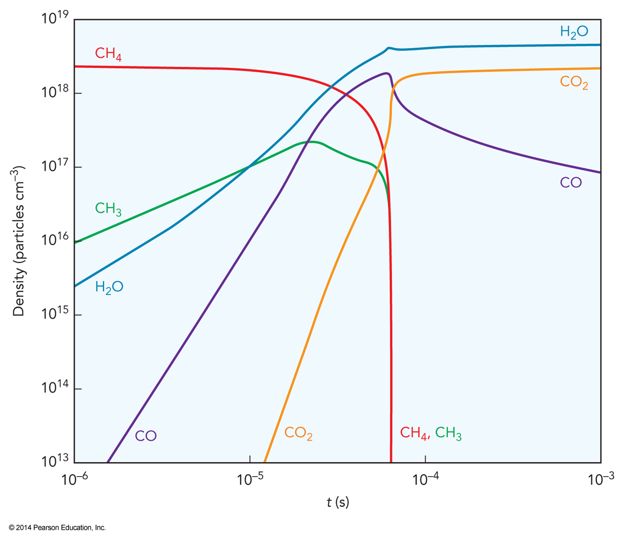
- An ideal Bunsen burner would provide a laminar flame in which the \(\chem{CH_4}\) entering the conbusion region is completely oxidized to \(\chem{H_2O}\) and \(\chem{CO_2}\)
- The principle elementary reactions relevant to this process are given in the following tables - there are other secondary elementary reactions possible
- The shear number of elementary reactions makes analyzing the kinetics daunting so we need a way of simplifying things
- Of all the reactants and products, only seven are chemically stable: \( \chem{CH_4,\,O_2,\,H_2O,\,CO_2,\,CO,\,H_2,\,CH_2O} \)
Important Reactions in the Combusion of \(\chem{CH_4}\) in \(\chem{O_2}\)
These reaction rates are determined at 2000 K in units of \(\left( \chem{cm^{3}\,mol^{-1}} \right)^{n-1}\,\chem{s}^{-1}\), when \(n\) is the molecularity of the reaction. When \(k_r\) is not given, the reverse reaction is negligible.
| reaction | \(k_f\) | \(k_r\) | |
|---|---|---|---|
| 1. | \( \chem{H+O_2 \rightleftharpoons OH+O} \) | \( 2.92 \times 10^{11} \) | \( 1.15 \times 10^{13} \) |
| 2. | \( \chem{H+O_2+M \rightleftharpoons HO_2+M} \) | \( 5.26 \times 10^{15} \) | \( 2.17 \times 10^{10} \) |
| 3. | \( \chem{H_2+O \rightleftharpoons H+OH} \) | \( 8.97 \times 10^{12} \) | \( 7.02 \times 10^{12} \) |
| 4. | \( \chem{H_2+OH \rightleftharpoons H+H_2O} \) | \( 8.34 \times 10^{12} \) | \( 8.36 \times 10^{11} \) |
| 5. | \( \chem{2OH \rightleftharpoons H_2O+O} \) | \( 8.48 \times 10^{12} \) | \( 1.20 \times 10^{12} \) |
| 6. | \( \chem{HO_2+H \rightleftharpoons 2OH} \) | \( 1.17 \times 10^{14} \) | \( 6.00 \times 10^{8} \) |
Important Reactions in the Combusion of \(\chem{CH_4}\) in \(\chem{O_2}\) (cont.)
| reaction | \(k_f\) | \(k_r\) | |
|---|---|---|---|
| 7. | \( \chem{HO_2+H \rightleftharpoons H_2+O_2} \) | \( 2.10 \times 10^{13} \) | |
| 8. | \( \chem{HO_2+H \rightleftharpoons H_2O+O} \) | \( 1.95 \times 10^{13} \) | |
| 9. | \( \chem{HO_2+OH \rightleftharpoons H_2O+O_2} \) | \( 1.30 \times 10^{13} \) | |
| 10. | \( \chem{CO+OH \rightleftharpoons CO_2+H} \) | \( 4.74 \times 10^{11} \) | \( 2.01 \times 10^{11} \) |
| 11. | \( \chem{CH_4+H \rightleftharpoons H_2+CH_3} \) | \( 1.95 \times 10^{13} \) | \( 9.40 \times 10^{11} \) |
| 12. | \( \chem{CH_4+OH \rightleftharpoons H_2O+CH_3} \) | \( 7.37 \times 10^{12} \) | \( 1.05 \times 10^{11} \) |
| 13. | \( \chem{CH_3+O \rightleftharpoons CH_2O+H} \) | \( 7.00 \times 10^{13} \) | \( 5.30 \times 10^{7} \) |
| 14. | \( \chem{CH_3+OH \rightleftharpoons CH_2O+2H} \) | \( 1.83 \times 10^{13} \) |
Important Reactions in the Combusion of \(\chem{CH_4}\) in \(\chem{O_2}\) (cont. more)
| reaction | \(k_f\) | \(k_r\) | |
|---|---|---|---|
| 15. | \( \chem{CH_3+OH \rightleftharpoons CH_2O+H_2} \) | \( 8.00 \times 10^{12} \) | |
| 16. | \( \chem{CH_3+OH \rightleftharpoons CH_2+H_2O} \) | \( 4.26 \times 10^{12} \) | |
| 17. | \( \chem{CH_3+H \rightleftharpoons CH_2+H_2} \) | \( 4.07 \times 10^{12} \) | |
| 18. | \( \chem{CH_3+H+M \rightleftharpoons CH_4+M} \) | \( 1.11 \times 10^{17} \) | \( 4.30 \times 10^{7} \) |
| 19. | \( \chem{CH_2+H \rightleftharpoons CH+H_2} \) | \( 4.00 \times 10^{13} \) | \( 1.31 \times 10^{13} \) |
| 20. | \( \chem{CH_2+OH \rightleftharpoons CH_2O} \) | \( 2.50 \times 10^{13} \) | |
| 21. | \( \chem{CH_2+OH \rightleftharpoons CH+H_2O} \) | \( 2.11 \times 10^{13} \) | |
| 22. | \( \chem{CH_2+O_2 \rightleftharpoons CO_2+2H} \) | \( 4.45 \times 10^{12} \) |
Important Reactions in the Combusion of \(\chem{CH_4}\) in \(\chem{O_2}\) (completed)
| reaction | \(k_f\) | \(k_r\) | |
|---|---|---|---|
| 23. | \( \chem{CH_2+O_2 \rightleftharpoons CO+OH+H} \) | \( 4.45 \times 10^{12} \) | |
| 24. | \( \chem{CH+O_2 \rightleftharpoons CHO+O} \) | \( 3.00 \times 10^{13} \) | |
| 25. | \( \chem{CH+OH \rightleftharpoons CHO+H} \) | \( 3.00 \times 10^{13} \) | |
| 26. | \( \chem{CH_2O+H \rightleftharpoons CHO+H_2} \) | \( 9.16 \times 10^{12} \) | \( 4.20 \times 10^{9} \) |
| 27. | \( \chem{CH_2O+OH \rightleftharpoons CHO+H_2O} \) | \( 2.22 \times 10^{13} \) | \( 8.60 \times 10^{9} \) |
| 28. | \( \chem{CHO+H \rightleftharpoons CO+H_2} \) | \( 2.00 \times 10^{14} \) | \( 2.80 \times 10^{5} \) |
| 29. | \( \chem{CHO+OH \rightleftharpoons CO+H_2O} \) | \( 1.00 \times 10^{14} \) | \( 1.30 \times 10^{4} \) |
| 30. | \( \chem{CHO+M \rightleftharpoons CO+H+M} \) | \( 1.04 \times 10^{13} \) | \( 3.63 \times 10^{12} \) |
| 31. | \( \chem{CHO+O_2 \rightleftharpoons CO+HO_2} \) | \( 3.00 \times 10^{12} \) |
Simplifying the System
- We cannot simply neglect steps based on rate constant
- Reaction rates depend on reactant concentrations
- A reaction involving \(\chem{CH_4}\) will be much more important initially than a much faster reaction whose reactants are intermediates formed later in the reaction
- An analysis of the numerical results can identify the most important series of reactions and break them up into different categories
- The dominant chemistry of the methane flame can be described by the reduced set of multi-step reactions given on the following slides
- These different steps occur at different points in the flame (upcoming figure)
\(\chem{O_2}\) Consumption Steps
| 1. | \( \chem{2\left( H+O_2 \rightleftharpoons OH+O \right)} \) |
| 3. | \( \chem{2\left( H_2+O \rightleftharpoons H+OH \right)} \) |
| 4. | \( \chem{4\left( H_2+OH \rightleftharpoons H+H_2O \right)} \) |
| net | \( \chem{2\left( 3H_2+O_2 \rightleftharpoons 2H_2O+2H \right)} \) |
| \( \Delta_{rxn}H = -42.7\,\mathrm{kJ}\,\mathrm{mol}^{-1} \) | |
| \( \Delta_{rxn}S = 9.9\,\mathrm{kJ}\,\mathrm{K}^{-1}\,\mathrm{mol}^{-1} \) | |
\(\chem{CH_4}\) Consumption Steps
| 11. | \( \chem{CH_4+H \rightleftharpoons H_2+CH_3} \) |
| 13. | \( \chem{CH_3+O \rightleftharpoons CH_2O+H} \) |
| 26. | \( \chem{CH_2O+H \rightleftharpoons CHO+H_2} \) |
| 30. | \( \chem{CHO+M \rightleftharpoons CO+H+M} \) |
| 3. | \( \chem{H+OH \rightleftharpoons O+H_2} \) |
| 4. | \( \chem{H+H_2O \rightleftharpoons OH+H_2} \) |
| net | \( \chem{CH_4+2H+H_2O \rightleftharpoons CO+4H_2} \) |
| \( \Delta_{rxn}H = -229.8\,\mathrm{kJ}\,\mathrm{mol}^{-1} \) | |
| \( \Delta_{rxn}S = 115.9\,\mathrm{kJ}\,\mathrm{K}^{-1}\,\mathrm{mol}^{-1} \) | |
\(\chem{CO}\) Shift Steps
| 10. | \( \chem{CO+OH \rightleftharpoons CO_2+H} \) |
| 4. | \( \chem{H+H_2O \rightleftharpoons H_2+OH} \) |
| net | \( \chem{CO+H_2O \rightleftharpoons CO_2+H_2} \) |
| \( \Delta_{rxn}H = -41.2\,\mathrm{kJ}\,\mathrm{mol}^{-1} \) | |
| \( \Delta_{rxn}S = -42.1\,\mathrm{kJ}\,\mathrm{K}^{-1}\,\mathrm{mol}^{-1} \) | |
\(\chem{H_2}\) Recombination Steps
| 2. | \( \chem{O_2+H+M \rightleftharpoons HO_2+M} \) |
| 9. | \( \chem{OH+HO_2 \rightleftharpoons H_2O+O_2} \) |
| 4. | \( \chem{H+H_2O \rightleftharpoons OH+H_2} \) |
| net | \( \chem{2H+M \rightleftharpoons H_2+M} \) |
| \( \Delta_{rxn}H = -453.9\,\mathrm{kJ}\,\mathrm{mol}^{-1} \) | |
| \( \Delta_{rxn}S = -98.7\,\mathrm{kJ}\,\mathrm{K}^{-1}\,\mathrm{mol}^{-1} \) | |
Schematic of the Regions in the Methane-Air Flame
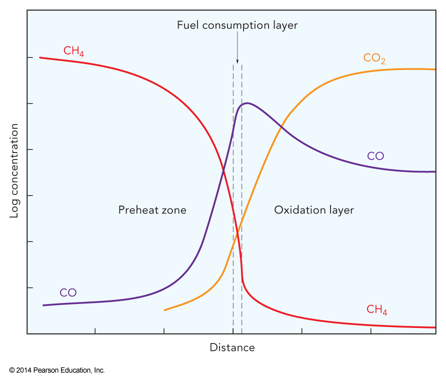 Note: It is possible to decrease the amount of \(\chem{CO}\) in the exhaust gases by increasing the initial \(\chem{O_2}\) concentration or by seeding the fuel mix with other sources of \(\chem{OH}\).
Astrophysics and Spectroscopy
- Physical chemistry and astrophysics share many common interest
- The greatest similarities rest with the coincidence of observational methods
- In both fields, the object of study is difficult to probe directly
- in physical chemistry it is often a chemical sample too small or too reactive to isolate
- in astrophysics it may be a star one thousand light years away
- Spectroscopy has worked well both both
Stellar Emission
- A star is a cloud of gas so massive and so dense that its own gravity compresses the matter at its core with enough force to enable nuclear fusion
- The core is the hottest and densest region of the star
- The star become cooler and more diffuse as the distance from the core increases
- The interior gas of a star is gas of ionized atoms, mainly hydrogen and helium, too hot and dense for the emitted radiation to show any individual spectroscopic transitions
The Parts of a Stellar Atmosphere
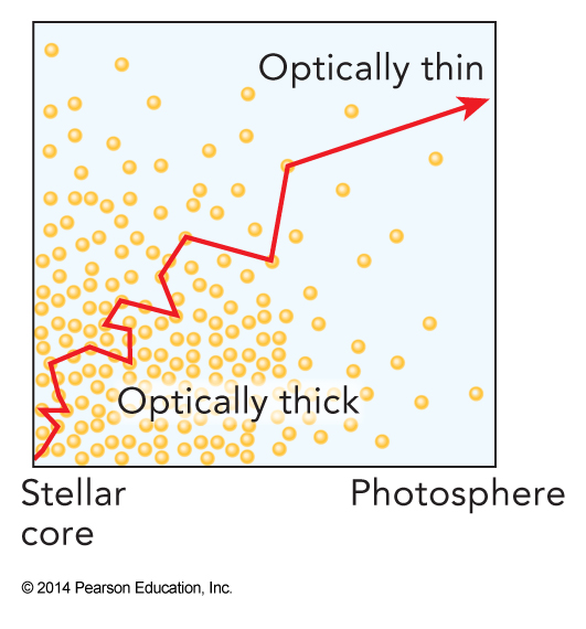
- In the inner part of the star, the matter density is so high over such a large distance that photons cannot leave without first being scattered or absorbed and re-emitted by these ions
- These regions can't be penetrated by radiation without interaction with the matter
- This type of region is called optically thick
- Photons emitted in the outer shell of a star find the matter density low enough that they can leave the star without more scattering or absorption
- This region of the star is essentially transparent to radiation
- This type of region is called the photosphere of the star and is optically thin
Optical Thickness of a Stellar Interior
Example 14.4
The sun's emission spectrum is characteristic of a blackbody at a temperature of 5800 K. find the peak emission wavelength. The blackbody radiaton spectrum is given by $$ \rho(\nu)\,d\nu = \frac{8\pi h\nu^3\,d\nu}{c^3\left( e^{\bfrac{h\nu}{k_BT}}-1 \right)} $$
Example 14.5
Heat is carried to the optically thin layer of a star primarily by convection. Radiation is just too inefficient a process in the dense core. Use Einstein's diffusion equation $$ t\approx \frac{R^2}{6D} $$ to estimate the time required for a photon generated at the sun's center to diffuse out of the sun's core, a distance of \( 1.7\times 10^8\,\mathrm{m} \). Although the actual number density on the core approaches \(10^{26}\,\mathrm{cm}^{-3}\), the photons interact weakly with the matter, and have a mean free path of about \(0.1\,\mathrm{cm}\). Use the mean free path to estimate the diffusion constant $$ D=\frac{\lambda^2\gamma}{2} $$ where \(\lambda\) is mean free path, \(\gamma\) is the collision frequency.
The Interstellar Medium
- Most of the observable universe is believed to be interstellar gas and dust
- Within our galaxy, the number density of matter between stars varies between \(10^3\) and \(10^6\,\mathrm{cm}^{-3}\)
- Most of this matter is either \(\chem{H^+}\), \(\chem{H_2}\), or \(\chem{H}\)
- This matter is largely known as the interstellar medium
- The ionized gas corresponds to the largest, hotest, and sparsest regions of interstellar space
- The molecular hydrogen exists only in compact, cold, relatively dense clumps known as molecular clouds
- Molecular clouds are about \(10^{13}\) times less dense than our atmosphere
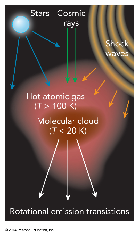
Energy Transfer in Molecular Clouds
Cosmic Abundances of the Dominant Elements, Relative to Hydrogen
| element | relative abundance | species in molecular clouds |
|---|---|---|
| \(\chem{H}\) | 1 | \(\chem{H,\,H_2,\,H_2O,\,HCN}\) |
| \(\chem{He}\) | \(6.3 \times 10^{-2}\) | \(\chem{He}\) |
| \(\chem{O}\) | \(6.9 \times 10^{-4}\) | \(\chem{CO,\,SiO,\,H_2O,\,OH,\,HCO,\,MgO,\,CO_2,\,OCS,\,O_2}\) |
| \(\chem{C}\) | \(4.2 \times 10^{-4}\) | \(\chem{CO,\,HCN,\,CS,\,HCO,\,CO_2,\,CH_4,\,OCS}\) |
| \(\chem{N}\) | \(8.7 \times 10^{-5}\) | \(\chem{N_2,\,HCN,\,NH_3,\,NH_2}\) |
| \(\chem{Si}\) | \(4.5 \times 10^{-5}\) | \(\chem{Si,\,SiS,\,SiO,\,SiO_2}\) |
| \(\chem{Mg}\) | \(4.0 \times 10^{-5}\) | \(\chem{Mg,\,MgH,\,MgS,\,MgO}\) |
| \(\chem{Ne}\) | \(3.7 \times 10^{-5}\) | \(\chem{Ne}\) |
| \(\chem{Fe}\) | \(3.2 \times 10^{-5}\) | \(\chem{Fe}\) |
| \(\chem{S}\) | \(1.6 \times 10^{-5}\) | \(\chem{SiS,\,CS,\,S,\,HS,\,H_2S,\,MgS}\) |
Interstellar Chemical Synthesis: Detected Organic Molecular
| \(\chem{CH}\) | \(\chem{C_2}\) | \(\chem{CN}\) | \(\chem{CO}\) | \(\chem{CS}\) |
| \(\chem{CH^+}\) | \(\chem{HOC^+}\) | \(\chem{HCS^+}\) | \(\chem{HCNH^+}\) | \(\chem{HCO^+}\) |
| \(\chem{HCN}\) | \(\chem{HNC}\) | \(\chem{HNCO}\) | \(\chem{HNCS}\) | |
| \(\chem{HC_3N}\) | \(\chem{HC_5N}\) | \(\chem{HC_7N}\) | \(\chem{HC_9N}\) | \(\chem{HC_{11}N}\) |
| \(\chem{CH_3CN}\) | \(\chem{CH_3NC}\) | \(\chem{C_2H_3CN}\) | \(\chem{C_3H_5CN}\) | |
| \(\chem{CH_3CHO}\) | \(\chem{HC_2CHO}\) | \(\chem{HC_3HOH}\) | \(\chem{CH_3CH_2OH}\) | \(\chem{CH_3OH}\) |
| \(\chem{C_3O}\) | \(\chem{HC_2O}\) | \(\chem{H_2CS}\) | \(\chem{HCOOH}\) | \(\chem{CH_3COOH}\) |
| \(\chem{CH_3SH}\) | \(\chem{NH_2CHO}\) | \(\chem{NH_2CN}\) | \(\chem{c-SiC_2}\) | \(\chem{c-C_3H_2}\) |
| \(\chem{C_3N}\) | \(\chem{CH_3C_3N}\) | \(\chem{CH_3C_4H}\) | \(\chem{CH_3CCH}\) | |
| \(\chem{C_2H}\) | \(\chem{C_3H}\) | \(\chem{C_4H}\) | \(\chem{C_5H}\) |
Example 14.9
Based on the parameters given in the following table, estime the rates of formation of \(\chem{HCl^+}\) and \(\chem{HCl}\) at 80 K in the Orion Molecular Cloud from the reactions given. $$ \begin{align} \chem{Cl^++H_2} &\rightarrow^{k_1} \chem{HCl^++H} \\ \chem{Cl+H_2} &\rightarrow^{k_2} \chem{HCl+H} \end{align} $$
| \( \conc{Cl^+} \) | \( 1 \times 10^{-12} \,\mathrm{cm}^{-3} \) | \( \conc{Cl} \) | \( 4 \times 10^{-3} \,\mathrm{cm}^{-3} \) |
| \( \conc{H_3^+} \) | \( 1 \times 10^{-4} \,\mathrm{cm}^{-3} \) | \( \conc{H_2} \) | \( 1 \times 10^{5} \,\mathrm{cm}^{-3} \) |
| \( \conc{e^-} \) | \( 1 \times 10^{-12} \,\mathrm{cm}^{-3} \) | \( T \) | \( 80\,\mathrm{K} \) |
| \( A_1(80\,\mathrm{K}) \) | \( 1 \times 10^{-9} \,\mathrm{cm}^{-3}\,\mathrm{s}^{-1} \) | \( A_2(80\,\mathrm{K}) \) | \( 1 \times 10^{-10} \,\mathrm{cm}^{-3}\,\mathrm{s}^{-1} \) |
| \( E_{a1} \) | \( 0 \,\mathrm{kJ}\,\mathrm{mol}^{-1} \) | \( E_{a2} \) | \( 23 \,\mathrm{kJ}\,\mathrm{mol}^{-1} \) |
Example 14.10
Contraryto the apparent results of the previous example, the \(\bfrac{\conc{HCl}}{\conc{HCl^+}}\) ratio in the Orion Molecular Cloud is estimated at \( 2 \times 10^9 \). There is a more efficient way to produce the \(\chem{HCl}\) than by reaction 2 in the previous mechanism, and the \(\chem{HCl^+}\) is itself consumed in one of those reactions: $$ \begin{align} \chem{Cl+H_3^+ \xrightarrow{k_3} HCl^++H_2} &~~~~~~~~& k_3 &= 1.0 \times 10^{-9}\,\mathrm{cm}^3\,\mathrm{s}^{-1} \\ \chem{HCl^++H_2 \xrightarrow{k_4} H_2Cl^++H} &~~~~~~~~& k_4 &= 1.3 \times 10^{-9}\,\mathrm{cm}^3\,\mathrm{s}^{-1} \\ \chem{H_2Cl^++e^- \xrightarrow{k_5} HCl+H} &~~~~~~~~& k_5 &= 1.5 \times 10^{-7}\,\mathrm{cm}^3\,\mathrm{s}^{-1} \end{align} $$ Reaction 3 is actually about four times more efficient at forming \(\chem{HCl^+}\) than reaction 1 (but doesn't offer such a straightfoward comparison with neutral-neutral kinetics). The net reaction is $$ \chem{Cl+H_3^++e^- \rightarrow HCl+2H} $$ Find the steady-state number density of \(\chem{HCl^+}\) in this mechanism, using the parameters from our previous example.
/