Mass Transport: Collisions and Diffusion
Shaun Williams, PhD
Collision Parameters
Chemical Environments
- Chemistry study solids and liquids
- Densities of over \(10^{22}\) particles per cubic centimeter
- They also study interstellar nebular
- Densities of \(\lt 10^3\) particles per cubic centimeter
- We need to identify key parameters that can be used to define any system
Molecular Collisions
- The most common parameters used to describe collisions between two molecules
- Distribution of molecular velocities
- Average collision energy
- Effective cross-sectional area ("collision cross section")
- Average collision frequency
- Average distance a molecule travels between collisions ("mean free path")
Molecular Speeds
- The distribution of molecular speeds in our canonical sample obey a Maxwell-Boltzmann distribution
- Any statistical average as three characteristic values:
- The mean (average)
- The mode (having the highest probability)
- The median (half population above and half below)
Various Maxwell-Boltzmann Speeds
- From chapter 3: \( \expect{v} = \sqrt{\frac{8k_\mathrm{B}T}{\pi m}} \)
- We can determine the mode $$ \begin{align} 0 &= \frac{d\mathcal{P}_v(v)}{dv} = \left( \frac{2m^3}{\pi k_\mathrm{B}^3T^3} \right) \left[ \begin{split} & 2ve^{-\frac{mv^2}{2k_\mathrm{B}T}} \\ & +v^2 e^{-\frac{mv^2}{2k_\mathrm{B}T}} \left( -\frac{m}{2k_\mathrm{B}T} \right) \left( 2v \right) \end{split} \right] \\ v_\chem{mode} &= \sqrt{\frac{2k_\mathrm{B}T}{m}} \\ v_\chem{med} &= 1.538 \sqrt{\frac{k_\mathrm{B}T}{m}} \end{align} $$
Average Relative Speed
- The average relative speed is the crucial quantity for molecular collisions
- For a generic molecules A and B $$ \expect{v_\chem{AB}} = \sqrt{\frac{8k_\mathrm{B}T}{\pi \mu}} $$
- If the two molecules are the same then $$ \expect{v_\chem{AA}} = \sqrt{\frac{16k_\mathrm{B}T}{\pi m}} = \sqrt{2} \expect{v} $$
Root Mean Squared Velocity
- Particles are equally likely to travel in any direction
- This means that \( \expect{\vec{v}}=0 \)
- Due to this we define the rms velocity $$ \begin{align} v_\chem{rms} &\equiv \left( \expect{v^2} \right)^\bfrac{1}{2} = \left( 3 \expect{v_x^2} \right)^\bfrac{1}{2} \\ &= \sqrt{\frac{3k_\mathrm{B}T}{m}} \end{align} $$
Collision Energy
- The collision energy is the energy of a pair of colliding particles relative to the potential energy when the two particles are separated by a large distance
- We may believe that we need to worry about the frame of reference we use
- The collision energy is the same regardless of whether the frame of reference is moving or not
Frame of Reference
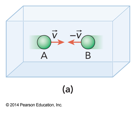 $$ K = 2\left( \frac{1}{2} mv^2 \right) = mv^2 $$
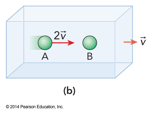 $$ K = \left( \frac{1}{2} m\left( 2v \right)^2 \right) = 2mv^2 $$
So what do we use?
- The kinetic energy relevant to collision strength is measured in the center of mass reference frame
- The frame in which the center of mass is at rest
- For two particles A and B, the collision energy is \( \frac{\mu v_\chem{AB}^2}{2} \) $$ \expect{E_\chem{AB}} = \frac{\mu \expect{v_\chem{AB}}^2}{2} = \frac{\mu \left( 3k_\mathrm{B}T \right)}{2\mu} = \frac{3k_\mathrm{B}T}{2} $$
- Note: from chapter 3: \( \expect{v_x^2} = \frac{k_\mathrm{B}T}{m} \)
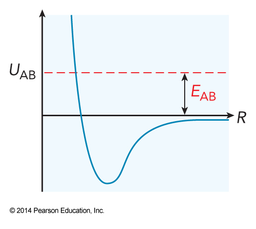
Intermolecular Potential Energy Surface with \(E_\chem{AB}\)
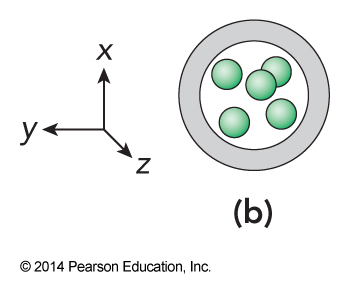
Collision Cross Section
- Expresses the maximum separation between interacting molecules in the form of an area.
Selected Collision Cross Sections, \( \sigma \left( \AA^2 \right) \)
| Gas | \( \sigma (\AA^2) \) | Gas | \( \sigma (\AA^2) \) |
|---|---|---|---|
| \( \chem{He} \) | 22 | \( \chem{Ne} \) | 25 |
| \( \chem{H_2} \) | 27 | \( \chem{Ar} \) | 36 |
| \( \chem{O_2} \) | 36 | \( \chem{N_2} \) | 37 |
| \( \chem{NH_3} \) | 43 | \( \chem{CO_2} \) | 45 |
| \( \chem{CH_4} \) | 52 | \( \chem{H_2O} \) | 62 |
| \( \chem{C_2H_4} \) | 71 | \( \chem{C_2H_2} \) | 72 |
| \( \chem{C_2H_6} \) | 84 | \( \chem{SO_2} \) | 90 |
| \( n-\chem{C_4H_{10}} \) | 148 | \( \chem{CHCl_3} \) | 156 |
Collision Cross Section of Dissimilar Molecules
$$ \begin{align} \sigma_\chem{AB} &= \pi d_\chem{AB}^2 = \pi \left( \frac{d_\chem{A}+d_\chem{B}}{2} \right)^2 \\ &= \frac{\pi}{4} \left( d_\chem{A}^2 + 2d_\chem{A}d_\chem{B} + d_\chem{B}^2 \right) \\ &= \frac{\pi}{4} \left( \frac{\sigma_\chem{A}}{\pi} + \frac{2\sqrt{\sigma_\chem{A}\sigma_\chem{B}}}{\pi} + \frac{\sigma_\chem{B}}{\pi} \right) \\ &= \frac{1}{4} \left( \sigma_\chem{A} + 2\sqrt{\sigma_\chem{A}\sigma_\chem{B}} + \sigma_\chem{B} \right) \end{align} $$
Average Collision Frequency
- The number of particles in the path of a reference particle is \( N_\chem{coll} = \rho \sigma l \)
- The collision frequency is related to time it takes the reference particle to travel the distance \(l\) $$ \gamma = \frac{N_\chem{coll}}{\Delta t_\chem{coll}} = \frac{\rho \sigma l}{\bfrac{l}{\expect{v_\chem{AA}}}} = \rho \sigma \expect{v_\chem{A}} $$
Mean Free Path
- The average distance a particle travels between collisions
- Given by the average speed divided by the average collision frequency $$ \lambda = \frac{\expect{v}}{\gamma} = \frac{1}{\sqrt{2}\rho \sigma} $$
Example 5.1
What are \(\rho\), \(\lambda\), \(\expect{v_\chem{AA}}\), and \(\lambda\) for \(\chem{N_2}\) at \(1.00\,\mathrm{bar}\) and \(298\,\mathrm{K}\)? What is the average collision energy in units of \(\chem{cm^{-1}}\)?
Changes in Trajectory
- So far we evaluated equation independent of the change in the particles trajectory after each collision
- We need to know how far, averaged over all these collisions, the molecules will travel
- We will fall back on statistical mechanics to determine how far, in any direction, a given molecule will travel after \(N_\chem{coll}\) collisions
The Random Walk
Randomness
- Oddly, randomness makes our task more manageable
- We have a classic random walk problem
- For random walk problems
- An atoms travels along a single line, suffering a collision at regular intervals
- For each collision, the atom either continues or reverses direction
- After \(N\) collisions, how far has the atom traveled?
Flipping a Coin
- Let’s treat the molecule collisions as flipping a coin \(N\) times
- Heads means moving forward one step
- Tails means moving backward one step
- Our progress is the number of times we get heads, \(i\), minus the number of times we get tails, \(j\) $$ k=i-j\;\text{and}\;N=i+j $$
- The coin flipping in random so many different \(k\)’s
Doing Some Math
$$ \mathcal{P}(k)=\frac{N!}{2^Ni!j!} $$
| $$ \begin{align} i &= N-j=N-(i-k) \\ &= N-i+k \\ i &= \frac{N+k}{2} \end{align} $$ | $$ \begin{align} j &= N-i=N-(j+k) \\ &= N-i-k \\ j &= \frac{N-k}{2} \end{align} $$ |
$$ \mathcal{P}(k) = \frac{N!}{2^N \frac{N+k}{2}!\frac{N-k}{2}!} $$
More Math
- Due to the size of \(N\), this equation become unwieldy so we use some approximations $$ \ln \mathcal{P}(k) = \ln N! - N\ln 2 - \ln \frac{N+k}{2}! - \ln \frac{N-k}{2}! $$
- We can simplify using Stirling’s approximation \( \ln N! \approx N\ln N - N \)
- Therefore $$ \ln \mathcal{P}(k) \approx N\ln N - \frac{1}{2} \left[ \begin{split} & (N+k)\ln (N+k) \\ & +(N-k) \ln (N-k) \end{split} \right] $$
Skipping Some More Math
- After performing another approximation and doing quite a bit of algebra we arrive at $$ \ln \mathcal{P}(k) \approx -\frac{k^2}{2N} $$
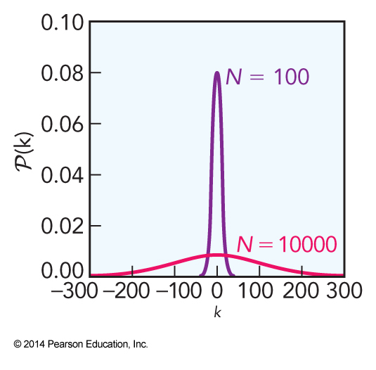
- Undoing the logarithm and normalizing the result we find that $$ \mathcal{P}(k) \approx \sqrt{\frac{2}{\pi N}} e^{-\frac{k^2}{2N}} $$
\(\mathcal{P}(k)\) Versus \(k\) for \(N=100\) and \( N=1000\)
Similar Equations
- We can rewrite our equation in terms of distance $$ \begin{align} \mathcal{P}_x(x) &= \frac{1}{\sqrt{2\pi}L} e^{-\frac{x^2}{2L^2}} \\ \mathcal{P}_V(x,y,z) &= \mathcal{P}_x(x)\mathcal{P}_y(y)\mathcal{P}_z(z) = \frac{1}{\sqrt{8\pi^3}L^3} e^{-\frac{x^2+y^2+z^2}{2L^2}} \\ \mathcal{P}_r(r) &= \frac{4\pi}{\sqrt{8\pi^3}L^3} e^{-\frac{r^2}{2L^2}} r^2 \end{align} $$
Transport without External Forces
Wandering Particles
- Particle tend to wander in containers
- A substance is isolated on one side of a container by a wall
- When the wall is removes the substance will begin to move throughout the entire container
- If we wait long enough, the substance will be fully mixed throughout the container
- This is due to random elastic collisions - diffusion
Diffusion
- Assume the bath (substance we are diffusing into) is a liquid or a gas
- We want the density as a function of time
- The width \(L\) of the distribution is \(\sqrt{N_\chem{coll}}\lambda\) in each direction
- From this we can find that \(L^2=\lambda^2 \gamma t\) $$ \mathcal{P}_r(r,t) = \frac{4\pi}{\sqrt{8\pi^3}\lambda^3} e^{-\frac{r^2}{2\lambda^2 \gamma t}} r^2 $$
Diffusion Equation
- We typically write the previous equation in terms of the diffusion constant $$ \begin{align} D &= \frac{\lambda^2\gamma}{2} = \frac{\expect{v_\chem{AA}}}{2\rho\sigma} = \frac{L^2}{2t} \\ \mathcal{P}_r(r,t) &= \frac{\pi}{2\left(\pi Dt\right)^\bfrac{3}{2}} e^{-\frac{r^2}{4DT}} r^2 \end{align} $$
- For molecule B diffusing through molecule A $$ D_\chem{B:A} \equiv \frac{\expect{v_\chem{AB}}}{2\rho_\chem{A}\sigma_\chem{AB}} = \frac{1}{2}\lambda \expect{v_\chem{B}} $$
Distance Travelled
- We can use our probability in a root mean square distance travelled during diffusion $$ \expect{x^2} = \int_0^\infty r^2 \mathcal{P}_r(r,t)\,dr = 6Dt $$
- This yields Einstein’s equation for diffusion $$ r_\chem{rms} = \expect{r^2}^\bfrac{1}{2} = \sqrt{6Dt} $$
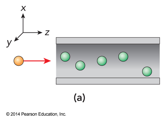
System for Fick's Laws
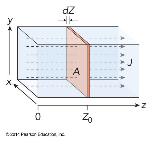
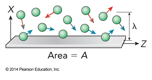
Fick's Laws
- The flux, \(J(z)\), is the rate at which mass flows through a given cross-sectional area
- Fick’s first law gives $$ J(z_0) = -D \left. \left( \frac{d\rho}{dz} \right) \right|_{z_0} $$
- Fick’s second law gives the change in the number density $$ \frac{d\rho}{dt} = D\frac{d^2\rho}{dz^2} $$
Example 5.2
Find the flux \(J(Z)\) and the flow rate \(\frac{d\rho}{dt}\) if the concentration is given by the linear gradient $$ \rho(Z) = \rho_0 cZ $$
Diffusion in Solids
- Molecules can diffuse through and across the surface of solids
- Note: \(r\) is now the distance along the surface $$ \mathcal{P}_r(r,t) = \frac{1}{2Dt} e^{-\frac{r^2}{4Dt}} r $$
Viscosity
- Fluids flow much slower than the particle velocity
- There are attractive forces between particles
- Inter-particle repulsive force allows particles to exchange momentum
- These correspond to viscosity, the resistance to flow
- We will start with hard spheres that only have the repulsive force
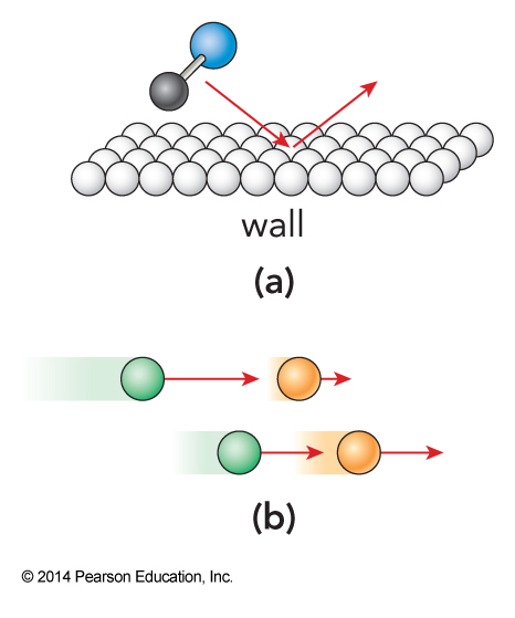
Momentum Transfer
System for Elementary Viscosity Law
Simple Viscosity
- The number of collisions that take place in an area of the wall in some time is $$ \begin{align} N_\chem{coll} &= \frac{\text{number of colliding particles in volume}}{\text{time per collision}} \Delta t \\ &= \frac{\rho A \frac{\lambda}{2}}{\frac{\lambda}{\expect{v_x}}} \Delta t = \frac{\rho A \expect{v_x} \Delta t}{2} \end{align} $$
How Does the Momentum Change per Collision?
- Remember from physics that \(\Delta p_i = m\Delta v_i\) $$ \Delta v_i = \Delta x \frac{\Delta v_i}{\Delta x} \approx \Delta x \frac{dv_i}{dx} $$
- We can set the change in \(x\) to the distance between collisions, which is the mean free path $$ \begin{align} \Delta v_i &\approx \lambda \frac{dv_i}{dx} \\ \Delta p_i &= m\lambda \frac{dv_i}{dx} \end{align} $$
Viscosity is a Force
- Viscosity is a force so $$ \begin{align} F &= ma = m\frac{dv}{dt} = \frac{d(mv)}{dt} = \frac{dp}{dt} \approx \frac{\Delta p}{dt} \\ F_\chem{viscosity} &\approx \frac{\Delta p}{\Delta t} = \left( \frac{\rho A\expect{v_x}}{2}\right) \left(m\lambda\frac{dv}{dx}\right) \equiv \eta A\frac{dV}{dx} \end{align} $$
- \(\eta\) is the viscosity
Solving the Viscosity
- For flow in one direction we have $$ \eta = \frac{1}{2}\rho \expect{v_x} m\lambda = \frac{1}{2}\rho \sqrt{\frac{8k_\mathrm{B}T}{\pi m}}m \left(\frac{1}{\rho \sigma}\right)=\sqrt{\frac{2mk_\mathrm{B}T}{\pi \sigma^2}} $$
Stokes' Law
- For a solvent with viscosity, \(\eta\), the speed \(v\) of a sphere of radius \(r\) (large compared to the molecular dimensions of the solvent) will meet a resisting force of $$ F_\chem{viscosity} = -6\pi \eta rv $$
Poiseuille's Formula
- For a viscous fluid flowing through a tube of radius \(r\) with pressure drop \(\Delta P\) over a distance \(l\), the volume flow rate is $$ \frac{dV}{dt} = \frac{\pi r^4 \Delta P}{8\eta l} $$
Example Diffusion Constants and Viscosities
| Sample | \(D_\chem{obs}\) | \(D_\chem{calc}\) | Sample | \(D_\chem{obs}\) | \(D_\chem{calc}\) |
|---|---|---|---|---|---|
| \(\chem{H_2}\text{ in }\chem{N_2} \\ \text{293.15 K, 1.01 bar}\) | \(0.772\) | \(1.06\) | \(\chem{H_2} \\ \text{300 K, 0.01 bar}\) | \(9.0\times 10^{-5}\) | \(10.8\times 10^{-5}\) |
| \(\chem{Ar}\text{ in }\chem{N_2} \\ \text{293.15 K, 1.01 bar}\) | \(0.190\) | \(0.312\) | \(\chem{Ar} \\ \text{300 K, 1.00 bar}\) | \(22.9\times 10^{-5}\) | \(36.3\times 10^{-5}\) |
| \(\chem{Ar}\text{ in }\chem{N_2} \\ \text{573.15 K, 1.01 bar}\) | \(0.615\) | \(0.853\) | \(\chem{Ar} \\ \text{600 K, 1.00 bar}\) | \(39.0\times 10^{-5}\) | \(50.8\times 10^{-5}\) |
| \(\chem{H_2O}\text{ in }\chem{N_2} \\ \text{293.15 K, 1.01 bar}\) | \(0.242\) | \(0.290\) | \(\chem{H_2O} \\ \text{300 K, 0.10 bar}\) | \(10.0\times 10^{-5}\) | \(14.3\times 10^{-5}\) |
| \(\chem{H_2O}\text{ in }\chem{acetone(liq)} \\ \text{298 K}\) | \(4.56\times 10^{-5}\) | \(4.7\times 10^{-4}\) | \(\chem{H_2O(liq)} \\ \text{298 K}\) | \(8.90\times 10^{-3}\) | \(14.3\times 10^{-5}\) |
Transport with External Forces
Sedimentation
- Typically gravity doesn’t play a role with small molecules and atoms
- Large molecules can be effected however
- Sedimentation uses gravity to separate compounds by different masses in solution
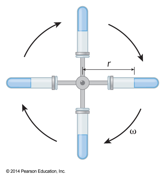
- Ultracentrifuges effectively increase the effective force of gravity
Schematic of Ultracentrifuge
Frictional Force
- For molecules that obey Stokes’ law, we can write a more general friction force law \(F_\chem{viscosity}=-fv\)
- \(f\) is the frictional force
- Ultracentrifuges use angular velocity to increase the force $$ F_\chem{cent} = (m-m_0) \omega^2 r \equiv m\omega^2 rb,\, b\equiv \left(1-\frac{m_0}{m}\right) $$
- \(b\) is the buoyancy correction
Simplifying
- At a steady state speed, \(v_\chem{ss}\) $$ v_\chem{ss} = \frac{m\omega^2 rb}{f} $$
- Another definition of the diffusion constant $$ D=\frac{k_\mathrm{B}T}{f} $$
- This makes the steady state velocity $$ v_\chem{ss} = \frac{m\omega^2 rbD}{k_\mathrm{B}T} $$
Electrophoresis
- Electrostatic force is opposed by viscosity
- The mobility of the molecules through the gel goes as \(v \propto \ln m\)
- So mixtures can be separated based on molecular masses
- Both electrophoresis and sedimentation are somewhat fallible because the mobility of particles is effected by shape
Convection and Chromatography
- Convection is the net flow of a gas or liquid sample, usually through some other fluid medium
- The medium must be macroscopically distinguishable from the sample
- For a tube laying parallel to the \(z\) axis $$ \expect{v_\chem{conv}} \equiv \frac{dz}{dT} $$
- The distribution of sample in a chromatography column $$ \mathcal{P}_z(z,t) = \left(4\pi Dt\right)^{-\bfrac{1}{2}} e^{-\frac{\left(z-\expect{v_\chem{conv}}t\right)^2}{4Dt}} $$
/