Statistical Mechanics and Molecular Interactions
Shaun Williams, PhD
Molecular Interactions
Gas Phase
- Average distance between molecules is usually so large that intermolecular interactions can be neglected
- During compression, these interactions become more important
- Unless they are highly reactive, intermolecular forces tend to be weak
Intermolecular Potential Energy
- The intermolecular potential energy is zero when there are no interactions between the particles
- Repulsions correspond to positive contributions
- Attractions correspond to negative contributions
- The most important interaction is the repulsion between particles
- When molecules are crammed together the like charges repel each other
Repulsion
- The distance at which this repulsion becomes important is small
- Determined by the atomic radii
- \(u_\chem{repulsion}\approx Ae^{-\frac{2cR}{a_0}}\)
- If the two particles can react, then this represents the energy barrier that must be overcome
Attractions
- Attractions between non-reacting molecules are significant over a much smaller temperature range
- The thermal energy \(k_\mathrm{B}T\) can easily cancel the negative attractive contribution
- Lowering the temperature tends to bring molecules closer together, first forming clusters, then droplets, then the formation of a condensed phase
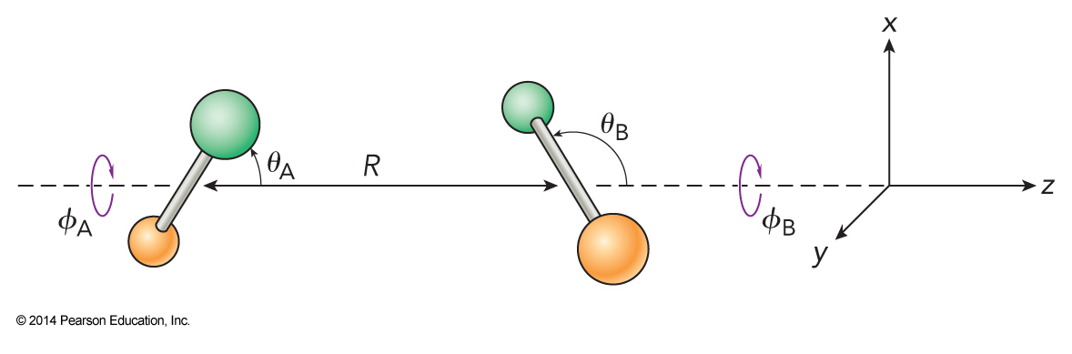
Dipole-Dipole Interaction
- One of the strongest of the attractive intermolecular forces is the dipole-dipole interaction
- The potential energy for the two rigid dipoles \(\mu_\chem{A}\) and \(\mu_\chem{B}\) interacting over distance \(R\) is $$ u_{2-2} = -\frac{2\mu_\chem{A}\mu_\chem{B}}{\left( 4\pi \varepsilon_0 \right)R^3}\left[ \begin{split} & \cos \theta_\chem{A} \cos \theta_\chem{B} \\ & - \frac{1}{2} \sin\theta_\chem{A} \sin\theta_\chem{B} \cos\left( \phi_\chem{A}-\phi_\chem{B} \right) \end{split} \right] $$
- Note: \(\phi=\phi_\chem{B}-\phi_\chem{A}\)
The Dipole-Dipole Interaction
Dipole-Dipole Interactions Continued
- If the two dipole moments both lie on the z axis $$ u=-\frac{2\mu_\chem{A}mu_\chem{B}}{\left( 2\pi \varepsilon_0 \right) R^3} $$
- In the liquid and gas phases, the dipole moments are not fixed in place, but rotate constantly
- We now need to determine how the average potential is governed
Beginning the Derivation
- In the gas phase, the molecules rotate through orientations of all types (attractive and repulsive)
- We need to average over all angles \(\theta_\chem{A}\), \(\theta_\chem{B}\), and \(\phi\) using the classical average value theorem $$ \expect{u} = \int \mathcal{P}(u)u\,d\tau $$
- The canonical distribution tells us that \(\mathcal{P}(u)\) will have the form $$ \mathcal{P}(u) = Ae^{-\frac{u}{k_\mathrm{B}T}} $$
Normalizing the Function
- \(A\) is the normalization constant $$ \begin{align} \int \mathcal{P}(u)\,d\tau &= A\int e^{-\frac{u}{k_\mathrm{B}T}}\, d\tau =1 \\ A &= \frac{1}{\int e^{-\frac{u}{k_\mathrm{B}T}}\,d\tau} \end{align} $$
- We can rewrite the average value equation $$ \expect{u} = A\int e^{-\frac{u}{k_\mathrm{B}T}} u\,d\tau = \frac{\int e^{-\frac{u}{k_\mathrm{B}T}}u\,d\tau}{\int e^{-\frac{u}{k_\mathrm{B}T}}\,d\tau} $$
Simplifying the Equation
- We need to use the following volume element to average away all the variables except \(R\) $$ d\tau' = \sin \theta_\chem{A} \,d\theta_\chem{A} \sin \theta_\chem{B} \,d\theta_\chem{B}\,d\phi $$
- Because \(u \ll k_\mathrm{B}T\) we can use a Taylor Series expansion \(\text{for }\left| x\right| \ll 1:\; e^x \approx 1+x\)
- This reduces our average potential energy to a simpler form
- After using a Taylor Series Expansion we have $$ \expect{u}_{\theta,\phi} = \frac{\int e^{-\frac{u}{k_\mathrm{B}T}}u\,d\tau'}{\int e^{-\frac{u}{k_\mathrm{B}T}}\,d\tau'} \approx \frac{\int \left( 1-\frac{u}{k_\mathrm{B}T} \right)u\,d\tau'}{\int \left( 1-\frac{u}{k_\mathrm{B}T} \right)\,d\tau'} = \dots = -\frac{2\mu_\chem{A}^2\mu_\chem{B}^2}{3R^6k_\mathrm{B}T} $$
Induced Dipole
- So far we have dealt with a permanent dipole moment on two molecules
- An electric field \(\varepsilon\) will induce a dipole moment
$$ \mu_\chem{induced} = \alpha \varepsilon $$
- \(\alpha\) is the polarizability of the molecule
- Dipole-induced dipole potential energy $$ u(R)=-\frac{4\mu_\chem{A}^2\alpha_\chem{B}}{\left( 4\pi \varepsilon_0 \right)R^6} $$
Dispersion Force
- Non-polar molecules a weak attractive force called the dispersion force
$$ u_\chem{disp} \equiv E_\chem{disp} \approx -\frac{\alpha^2 \Delta E}{2R^6} $$
- Where \(\Delta E\) is the separation between the ground and lowest excited state of the molecule.
- Notice that all the attraction interactions are proportional to \(-\frac{1}{R^6}\)
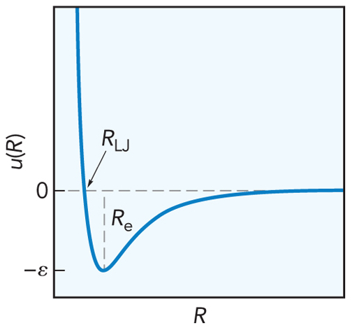
Model #1
- The most sophisticated model is the Lennard-Jones potential $$ \begin{align} u_\chem{LJ}(R) &= \varepsilon\left[ \left( \frac{R_e}{R} \right)^{12} - 2 \left( \frac{R_e}{R} \right)^6 \right] \\ \text{or} \\ u_\chem{LJ}(R) &= 4\varepsilon\left[ \left( \frac{R_\chem{LJ}}{R} \right)^{12} - \left( \frac{R_\chem{LJ}}{R} \right)^6 \right] \end{align} $$
The Lennard-Jones Potential
Model #2
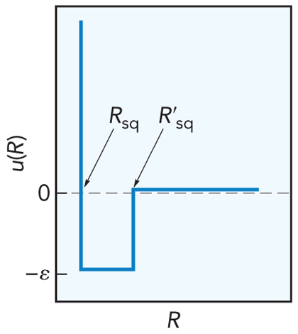
- The square well potential contains
- An impenetrable region
- An attractive region
- Interactions are turned off at long range
$$ u_\chem{sq}(R) = \begin{cases}
\infty & \text{if $R\le R_\chem{sq}$} \\
-\varepsilon & \text{if $R_\chem{sq}\lt R \le R'_\chem{sq}$} \\
0 & \text{if $R>R'_\chem{sq}$}
\end{cases}
$$
Square Well Potential
Model #3
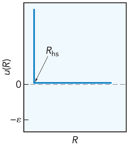
- The simplest model
- Particles modeled as hard spheres $$ u_\chem{hs} = \begin{cases} \infty & \text{if $R\le R_\chem{hs}$} \\ 0 & \text{if $R \gt R_\chem{hs}$} \end{cases} $$
Hard Sphere Model
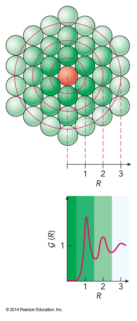
Solids
- The strength of the forces holding atoms together in a solid are great compared to the forces pushing atoms apart
- There are not any translations or rotations
- Those motions have been converted into vibrations
Liquids
- The most difficult phase to describe
- Molecules bound tightly enough to interact strongly, but not strongly enough to keep them fixed in position
- Descriptions of liquids usually rely on average properties of the structure
- Foremost is the pair correlation function \(\mathcal{G}(R)\) $$ \frac{\text{# of molecules at distance $R$}}{\text{# of molecules at distance R in random distribution}} $$
Pair Correlation Function
Pressure of a Non-Ideal Gas
Pressure of a Non-Ideal Gas
- Use methods developed in previous chapters to solve for the pressure of a non-ideal gas
- We need to solve the partial derivative $$ P=-\left( \frac{\partial E}{\partial V} \right)_{S,N} = \left( \frac{\partial E}{\partial S} \right)_{V,N} \left( \frac{\partial S}{\partial V} \right)_{E,N} $$
- The first term defines temperature
- The dependence on the intermolecular forces must be due to the last term
Entropy in a Non-Ideal Gas
- The entropy is determined by the ensemble size \(\Omega\)
- We need to determine how \(\Omega\) is affected by the intermolecular forces
- The degree of freedom is directly affected is translational motion
- The partition function $$ \mathcal{P}(E)=\Omega(E)\mathcal{P}(i) = \frac{\Omega(E)e^{-\frac{E}{k_\mathrm{B}T}}}{Q(T)} $$
Now Some Highlights of the Derivation
- The \(N\)-particle translational partition function for the ideal gas $$ Q_\chem{trans}(T,V) = \frac{1}{N!}\left( \frac{2\pi mk_\mathrm{B}T}{h^2} \right)^\bfrac{3N}{2} V^N $$
- The probability of the system being in any one translational state \(i\) that has energy \(E\) is $$ \mathcal{P}(i) = \frac{e^{-\frac{E}{k_\mathrm{B}T}}}{Q_\chem{trans}(T,V)}=\frac{1}{\Omega} $$
The Pressure of a Non-Ideal Gas
- After a lot of work we find that $$ \begin{align} P &= \frac{Nk_\mathrm{B}T}{V}-\frac{N^2k_\mathrm{B}T}{2V^2} \mathcal{I}(T) \\ &= \frac{nRT}{V}-\frac{n^2RT}{2V^2}\mathcal{N}_\mathrm{A} \mathcal{I}(T) \end{align} $$
- where $$ \mathcal{I}(T)\equiv V \int_0^1 \int_0^1 \int_0^1 \left( e^{-\frac{u(R)}{k_\mathrm{B}T}}-1 \right)\,dm_x\,dm_y\,dm_z $$
The Virial Expansion
- One of the two most common forms of the non-ideal gas law
- Writes the pressure as power series in the density $$ P=RT\left[ \frac{1}{V_m} + B_2(T)\frac{1}{V_m^2} \right] $$ where $$ B_2(T)\approx -\frac{1}{2}\mathcal{N}_\chem{A} \mathcal{I}(T) = -2\pi \mathcal{N}_\mathrm{A} \int_0^\infty \left( e^{-\frac{u(R)}{k_\mathrm{B}T}} -1 \right)R^2\,dR $$
Virial Expansion Continued
- There are higher order terms in the virial expansion $$ P = RT \left[ \frac{1}{V_m} + B_2(T)\frac{1}{V_m^2} + B_3(T)\frac{1}{V_m^3} + \dots \right] $$
- Ignoring terms past the second order we find that $$ V_m = \frac{RT}{2P}\left[ 1 + \sqrt{1+\frac{4B_2(T)P}{RT}} \right] $$
Virial Expansion Examples
| System | \(B_2\, @\, 273\,\mathrm{K} \\ (\mathrm{L\,mol^{-1}})\) | \(V_m\, @\, 1\,\mathrm{bar} \\ (\mathrm{L})\) | \(V_m\, @\, 10\,\mathrm{bar} \\ (\mathrm{L})\) |
|---|---|---|---|
| Helium | 0.0222 | 22.733 | 2.293 |
| Argon | -0.0279 | 22.683 | 2.243 |
| Ideal Gas | 22.711 | 2.271 |
The van der Waals Coefficients
- The second most common form of a non-ideal gas law
- Basically is a rewrite of the \(B_2(T)\) coefficients
- Doing some math we can arrive at $$ \begin{align} & B_2(T) \approx b-\frac{a}{RT} \\ & \text{where} \\ & b = \frac{2\pi \mathcal{N}_\chem{A} R_\chem{LJ}^3}{3} \text{ and } a=\frac{16\pi \mathcal{N}_\chem{A}^2\varepsilon R_\chem{LJ}^3}{9} \end{align} $$
- Plugging these values in and doing algebra we arrive at the traditional form $$ \left( P+\frac{a}{V_m^2}\right) \left(V_m-b\right) = RT $$
Lennard-Jones Parameters, van der Waals Coefficients, and Second Virial Coefficients
| Gas | \( \bfrac{\varepsilon}{k_\mathrm{B}} \\ (\mathrm{K}) \) | \( R_\chem{LJ} \\ (\mathrm{\AA}) \) | \( a \\ (\mathrm{L^2\,bar\,mol^{-1}}) \) | \( b \\ (\mathrm{L\,mol^{-1}}) \) | \( B_2(298\,\mathrm{K}) \\ (\mathrm{L\,mol^{-1}}) \) | \( B_2(298\,\mathrm{K})\text{(calc)} \\ (\mathrm{L\,mol^{-1}}) \) |
|---|---|---|---|---|---|---|
| \(\chem{He}\) | 10 | 2.58 | 0.0346 | 0.0238 | 0.012 | 0.020 |
| \(\chem{Ne}\) | 36 | 2.95 | 0.208 | 0.01672 | 0.011 | 0.022 |
| \(\chem{Ar}\) | 120 | 3.44 | 1.355 | 0.03201 | -0.016 | -0.004 |
| \(\chem{Kr}\) | 190 | 3.61 | 2.325 | 0.0396 | -0.051 | -0.042 |
| \(\chem{H_2}\) | 33 | 2.97 | 0.2453 | 0.02651 | 0.015 | 0.023 |
| \(\chem{N_2}\) | 92 | 3.68 | 1.370 | 0.0387 | -0.004 | 0.011 |
| \(\chem{O_2}\) | 113 | 3.43 | 1.382 | 0.03186 | -0.016 | -0.001 |
| \(\chem{CO}\) | 110 | 3.59 | 1.472 | 0.03948 | -0.008 | 0.001 |
| \(\chem{CO_2}\) | 190 | 4.00 | 3.658 | 0.04286 | -0.126 | -0.057 |
| \(\chem{CH_4}\) | 137 | 3.82 | 2.300 | 0.04301 | -0.043 | -0.016 |
| \(\chem{C_2H_2}\) | 185 | 4.22 | 4.516 | 0.05220 | -0.214 | -0.062 |
| \(\chem{C_2H_4}\) | 205 | 4.23 | 4.612 | 0.05821 | -0.139 | -0.080 |
| \(\chem{C_2H_6}\) | 230 | 4.42 | 5.570 | 0.06499 | -0.181 | -0.115 |
| \(\chem{C_6H_6}\) | 440 | 5.27 | 18.82 | 0.1193 | -1.454 | -0.542 |
Example 4.1
Estimate the van der Waals coefficient for helium and argon using their Lennard-Jones parameters.
Conversion to a Liquid
- As we compress a gas the particles get closer together
- Once the spacing becomes less than the average molecular size we expect the fluid to behave as a liquid
- We now need to look at the pair correlation function
The Pair Correlation Function
Pair Correlation Function
- The average number of molecules at distances between \(R_a\) and \(R_b\) is given as $$ \bar{N}_{R_a,R_b} = 4\pi \rho \int_{R_a}^{R_b} \mathcal{G}(R)R^2\,dR $$
- We can evaluate a function similar to the pair correlation function, \(\mathcal{P}_R(_{R12})\)
- The position probability distribution function per unit volume $$ \mathcal{P}_{V^N}(x_1,\dots,z_N) = \frac{e^{-\frac{U(x_1,\dots,z_N)}{k_\mathrm{B}T}}}{Q'_U(T,V)} $$
Position Probability Distribution Function
- After doing quite a bit of calculus we arrive at $$ \mathcal{P}_R(R)=\frac{4\pi R^2V\int_0^\infty \cdots \int_0^\infty e^{-\frac{U(x_1,\dots,z_N)}{k_\mathrm{B}T}}\,dx_3\dots dz_N}{Q'_U(T,V)} $$
- It turns out that $$ 4\pi \rho \int_{R_a}^{R_b} \mathcal{G}(R)R^2\,dR = \bar{N}_{R_a,R_b} = \left(N-1\right) \int_{R_a}^{R_b} \mathcal{P}_R(R)\,dR $$
- We can equate the integrands $$ \left(N-1\right) \mathcal{P}_R(R)\,dR = 4\pi \rho \mathcal{G}(R)R^2\,dR $$
Manipulating This Expression
$$ \begin{align} \mathcal{G}(R) &= \frac{N-1}{4\pi \rho R^2}\mathcal{P}_R(R) = \left( \frac{V(N-1)}{4N\pi R^2} \right) \mathcal{P}_R(R) \\ &= \left(\frac{V}{4\pi R^2}\right) \mathcal{P}_R(R) \\ &= \left(\frac{V}{4\pi R^2}\right) \frac{4\pi R^2V \int_0^a \cdots \int_0^c e^{-\frac{U}{k_\mathrm{B}T}}\,dx_3\dots dz_N}{Q'_U(T,V)} \\ &= \frac{V^2 \int_0^a \cdots \int_0^c e^{-\frac{U}{k_\mathrm{B}T}}\,dx_3\dots dz_N}{Q'_U(T,V)} \end{align} $$
More Manipulations
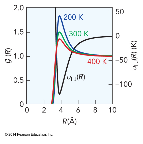
$$ \begin{align} \mathcal{G}(R) &= V^2 \frac{\int_0^a \cdots \int_0^c e^{-\frac{U}{k_\mathrm{B}T}}\,dx_3\dots dz_N}{\int_0^a \cdots \int_0^c e^{-\frac{U}{k_\mathrm{B}T}}\,dx_1\dots dz_N} \\ &= V^2 \frac{V^{N-2}e^{-\frac{u}{k_\mathrm{B}T}}\left[ 1+\frac{\mathcal{I}(T)}{V} \right]^{\frac{N(N+1)}{2}-1}}{V^N\left[ 1+\frac{\mathcal{I}(T)}{V} \right]^{\frac{N(N+1)}{2}}} \\ &= e^{-\frac{u(R)}{k_\mathrm{B}T}}\left[ 1+\frac{\mathcal{I}(T)}{V} \right]^{-1} \approx e^{-\frac{u(R)}{k_\mathrm{B}T}} \end{align} $$
Approximate Pair Correlation Function
Bose-Einstein and Fermi-Dirac Statistics
Indistinguishable Particles
- The wavefunction of a system of indistinguishable particles must be
- Antisymmetric to exchange for half-integer spin particles - Fermions
- Symmetric to exchange for integer spin particles – Bosons
- For an atom, if the total of # electrons, protons, and neutrons is even then it is a Boson
- \(\chem{{}^4He}\)
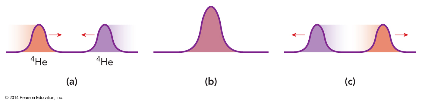
Helium-4
- Because it is a Boson lets consider a group of helium-4 atoms
- Let’s look at their translations
- They can all occupy the same quantum state
- This is non-classical because it means they all have the same position and velocity
Graphical Representation of Two Boson Wavefunctions
Counting States
- To evaluate the partition function we need to count states
- For fermions, this counting leads to Fermi-Dirac statistics
- For Bosons, this counting leads to Bose-Einstein statistics
Consider Two Particles Limited to Five Values
| \(I_b\) | |||||
|---|---|---|---|---|---|
| \(I_a\) | 1 | 2 | 3 | 4 | 5 |
| 1 | (11) | (12) | (13) | (14) | (15) |
| 2 | (21) | (22) | (23) | (24) | (25) |
| 3 | (31) | (32) | (33) | (34) | (35) |
| 4 | (41) | (42) | (43) | (44) | (45) |
| 5 | (51) | (52) | (53) | (54) | (55) |
Some States Are Available for Bosons But Not Fermions
- For Fermions $$ \Omega = \frac{g!}{N!(g-N)!} $$
- For Bosons $$ \Omega =\frac{(g+N-1)!}{N!(g-N)!} $$
- In these equations, there are \(g\) possible states for \(N\) particles
- At high temperatures, the spin statistics becomes irrelevant
Bose-Einstein Condensates
- There is a large disparity in the lab between liquid \(\chem{{}^3He}\) and \(\chem{{}^4He}\)
- \(\chem{{}^4He}\):
- At low temps, the number of accessible states is small, the chance that multiple atoms occupy the same quantum state is high (\(@\, 2.17\,\mathrm{K}\text{ and } 1\,\mathrm{bar}\))
- Liquid expands on cooling
- Thermal conductivity becomes discontinuous
- \(\chem{{}^3He}\):
- Exchange repulsion resists formation of the condensed phase more
- \(3.2\,\mathrm{K}\,\chem{{}^3He}\)
- \(4.22\,\mathrm{K}\,\chem{{}^4He}\)
- Exchange repulsion resists formation of the condensed phase more
- Because \(\chem{{}^4He}\) atoms do not repel each other strongly, liquid \(\chem{{}^4He}\) becomes a superfluid at temps below \(2.17\,\mathrm{K}\)
Superfluid \(\chem{{}^4He}\)
- Superfluids flow without significant resistance
- Even upward against gravity
- Superconductivity – also attributable to a similar manifestation of Bose-Einstein statistics
- In this case, pairs of electrons (called Cooper pairs) are the Bosons of the system
- Bose-Einstein statistics begin to dominate when $$ \rho_\mathrm{ps} = \rho \lambda_\chem{dB}^2 \gt 2.612 $$
Superfluidic Helium Video
/