Partitioning the Energy
Shaun Williams, PhD
Separation of Degrees of Freedom
Nuclear Motion
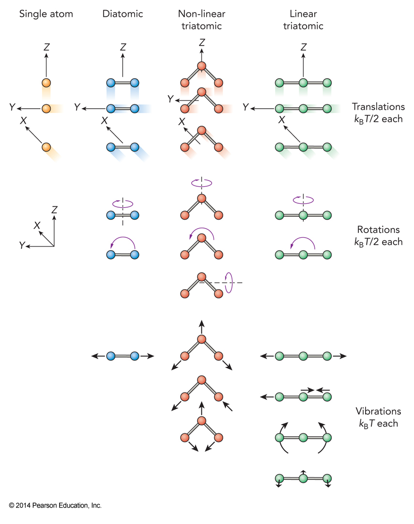
- For atoms in chemical bonds we can break down their nuclear motion into
- Translational – motion of the center of mass along \(x\), \(y\), or \(z\): 3 coordinates
- Rotational – changes in overall orientation of molecule: 2 angles for linear; 3 angles for nonlinear
- Vibrational – relative motions of the atoms: all remaining of the \(3N\) coordinates
Review of Canonical Ensemble
- Remember for the canonical ensemble $$ \begin{align} \mathcal{P}(\varepsilon) &= \frac{g(\varepsilon)e^{-\bfrac{\varepsilon}{k_\mathrm{B}T}}}{q(T)} \\ q(T) &= \sum_{\varepsilon=0}^{\infty} g(\varepsilon) e^{-\bfrac{\varepsilon}{k_\mathrm{B}T}} \end{align} $$
- We can break up the degeneracy \( g=g_\chem{vib}g_\chem{rot}g_\chem{trans} \)
- So, \( \varepsilon = \varepsilon_\chem{vib} + \varepsilon_\chem{rot} + \varepsilon_\chem{trans} \)
Evaluation of the Partition Function
- Adding our seperability to the partition function $$ \begin{align} q(T) &= \sum_{\varepsilon=0}^\infty g(\varepsilon)e^{-\frac{\varepsilon}{k_\mathrm{B}T}} = \sum_{\varepsilon_\chem{vib}}^\infty \sum_{\varepsilon_\chem{rot}}^\infty \sum_{\varepsilon_\chem{trans}}^\infty g_\chem{vib} g_\chem{rot} g_\chem{trans} e^{-\frac{\left(\varepsilon_\chem{vib}+\varepsilon_\chem{rot}+\varepsilon_\chem{trans}\right)}{k_\mathrm{B}T}} \\ &= \sum_{\varepsilon_\chem{vib}}^\infty \left[ g_\chem{vib} e^{-\frac{\varepsilon_\chem{vib}}{k_\mathrm{B}T}} \right] \sum_{\varepsilon_\chem{rot}}^\infty \left[ g_\chem{rot} e^{-\frac{\varepsilon_\chem{rot}}{k_\mathrm{B}T}} \right] \sum_{\varepsilon_\chem{trans}}^\infty \left[ g_\chem{trans} e^{-\frac{\varepsilon_\chem{trans}}{k_\mathrm{B}T}} \right] \\ &= q_\chem{vib} q_\chem{rot} q_\chem{trans} \\ \mathcal{P}(\varepsilon) &= \mathcal{P}_\chem{vib}\left( \varepsilon_\chem{vib}\right) \mathcal{P}_\chem{rot}\left( \varepsilon_\chem{rot}\right) \mathcal{P}_\chem{trans}\left( \varepsilon_\chem{trans}\right) \end{align} $$
Classical Average Value Theorem
- Measure a parameter \(A\left(\vec{s}\right)\) where \(\vec{s}\) are coords
- Find \(k\) different values
- Average value is $$ \expect{A} = \frac{\sum_i N_i A_i}{\sum_i N_i} = \sum_i \frac{N_i}{N} A_i = \sum_i \mathcal{P}\left(A_i\right) A_i $$
- \(A\) is a continuous parameter so this becomes $$ \expect{A} = \int_\text{all space} \mathcal{P}_\vec{s} \left(\vec{s}\right) A\left(\vec{s}\right)\, d\vec{s} $$
Moving Towards a Partition Function
- Let s be a single coordinates $$ \mathcal{P}\left( s_1 \le s < s_2 \right) = \int_{s_1}^{s_2} \mathcal{P}(s)\, ds = \int_{s_1}^{s_2} \frac{e^{-\frac{\varepsilon_s}{k_\mathrm{B}T}}}{q_s^`(T)}ds $$
- Note: \(q\)’s will have the same units as \(s\) $$ \begin{align} & \int_\text{all space} \mathcal{P}(s)\, ds = \int_\text{all space} \frac{e^{-\frac{\varepsilon_s}{k_\mathrm{B}T}}}{q_s^`(T)}ds = 1 \\ & \therefore q_s^`(T) = \int_\text{all space} e^{-\frac{\varepsilon_s}{k_\mathrm{B}T}}\, ds \end{align} $$
Translational Energy
- The total translational energy is $$ \frac{mv^2}{2} = \frac{mv_x^2}{2} + \frac{mv_y^2}{2} + \frac{mv_z^2}{2} $$
- The average translational energy $$ \begin{align} \expect{\frac{mv^2}{2}} &= \expect{\frac{mv_x^2}{2}+\frac{mv_y^2}{2}+\frac{mv_z^2}{2}} \\ &= \frac{m\expect{v_x^2}}{2} + \frac{m\expect{v_y^2}}{2} + \frac{m\expect{v_z^2}}{2} \end{align} $$
Probability of Translational Energies
- Probability of a particle having \(v_x\) $$ \begin{align} \expect{\varepsilon_x} &= \int_{-\infty}^{\infty} \mathcal{P}\left( v_x \right) \frac{mv_x^2}{2} \,dv_x \\ &= \frac{m}{2}\frac{\int_{-\infty}^{\infty}e^{-\frac{mv_x^2}{2k_\mathrm{B}T}} v_x^2 \,dv_x}{q_v^`(T)} \\ q_v^`(T) &= \int_{-\infty}^{\infty} e^{-\frac{mv_x^2}{2k_\mathrm{B}T}}\, dv_x \end{align} $$
Solving the Integral
- We can use integral tables to solve the integrals $$ \begin{align} & \int_0^\infty e^{-ax^2} \, dx = \frac{1}{2} \left( \frac{\pi}{a}\right)^{\bfrac{1}{2}} \\ & \int_0^\infty x^2 e^{-ax^2} \, dx = \frac{1}{4} \left( \frac{\pi}{a^3} \right)^\bfrac{1}{2} \end{align} $$
Manipulating These Expressions
$$ \begin{align} \int_{-\infty}^{\infty} x^2 e^{-ax^2}\,dx &= \int_{-\infty}^0 x^2 e^{-ax^2} \, dx + \int_0^\infty x^2 e^{-ax^2} \, dx \\ &= \int_0^\infty \left( -x \right)^2 e^{-a\left( -x\right)^2} \, dx + \int_0^\infty x^2 e^{-ax^2} \, dx \\ &= 2\int_0^\infty x^2 e^{-ax^2}\, dx = \frac{1}{2}\left( \frac{\pi}{a^3} \right)^\bfrac{1}{2} \\ \int_{-\infty}^\infty \, dx &= 2\int_0^\infty e^{-ax^2}\, dx = \left( \frac{\pi}{a} \right)^\bfrac{1}{2} \end{align} $$
Solving Out Energy Equations
$$ \begin{align} \expect{\varepsilon_x} &= \left( \frac{m}{2} \right) \frac{\int_{-\infty}^\infty e^{-\frac{mv_x^2}{2k_\mathrm{B}T}} v_x^2 \, dv_x}{\int_{-\infty}^\infty e^{-\frac{mv_x^2}{2k_\mathrm{B}T}} \, dv_x} \\ &= \left( \frac{m}{2} \right) \frac{\frac{1}{2} \left( \frac{\pi}{\left[ \frac{m}{2k_\mathrm{B}T} \right]^3} \right)^\bfrac{1}{2}}{\left( \frac{\pi}{\frac{m}{2k_\mathrm{B}T}} \right)^\bfrac{1}{2}} = \frac{m}{2}\frac{1}{2}\frac{2k_\mathrm{B}T}{m} = \frac{k_\mathrm{B}T}{2} \end{align} $$
Analysis
- An energy that varies as the square of its coordinate, \(\varepsilon_x=ax^2\), works out the same way $$ \expect{\varepsilon_x} = \frac{k_\mathrm{B}T}{a} $$
- The average value of \(x^2\) is $$ \expect{x^2} = \frac{1}{a} \expect{\varepsilon_x} = \frac{k_\mathrm{B}T}{2a} $$
- Now we know $$ \expect{\frac{mv^2}{2}} = \frac{m\expect{v_x^2}}{2} + \frac{m\expect{v_y^2}}{2} + \frac{m\expect{v_z^2}}{2} = \frac{3k_\mathrm{B}T}{2} $$
Rotations
- We can approximate the rotational energy $$ E_\chem{rot} = BJ \left( J+1 \right) \approx BJ^2 $$
- Every rotational coordinate, just like translations, has an approximate average energy of \( \frac{k_\mathrm{B}T}{2} \)
- Unfortunately, the vibrational considerations is different
Vibrations
- Consider vibrations where the thermal energy, \(k_\mathrm{B}T\), is large compared to the energy spacing in that coordinate
- Under this condition $$ \varepsilon_\chem{vib} = K+U = \frac{\mu v_\chem{vib}^2}{2} + \frac{k}{2}\left( R-R_e \right)^2 $$
- We solve this just like translations and rotations $$ \text{for }k_\mathrm{B}T \gg \omega_e:\; \expect{\varepsilon_\chem{vib}} = \frac{k_\mathrm{B}T}{2} + \frac{k_\mathrm{B}T}{2} = k_\mathrm{B}T $$
The Equipartition Principle
The Equipartition Principle
- \(N_\chem{ep}\) is the number of equipartition energy contributions $$ E=\\frac{1}{2}N_\chem{ep} Nk_\mathrm{B}T = \frac{1}{2} N_\chem{ep} nRT $$
- Note: \( R=\mathcal{N}_\mathrm{A} k_\mathrm{B} = 8.3145\, \chem{J\,K^{-1}\,mol^{-1}} \)
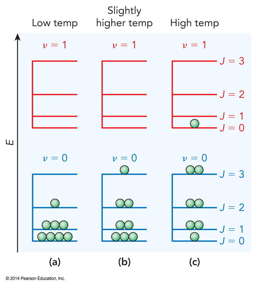
- At room temperature, all translations and rotations contribute to \(N_\chem{ep}\)
- At room temperature, only vibrations with roughly \( \omega_e < 300\, \chem{cm^{-1}} \) contribute to \(N_\chem{ep}\)
Motions Contributing to \(N_\chem{ep}\)
- For those vibrations that contribute to \(N_\chem{ep}\) $$ \begin{align} N_\chem{ep} = & \left( \text{number of translational degrees of freedom} \right) \\ & + \left( \text{number of rotational degrees of freedom} \right) \\ & + 2 \times \left( \text{number of vibrational degrees of freedom} \right) \end{align} $$
- At typical lab temperatures, few vibrational modes contribute to the number of equipartition degrees of freedom
- Vibrational spacings often more than 1000 K
Types of Gases
| Gas | Trans | Rotation | Vibration | Total Energy | |
|---|---|---|---|---|---|
| Monatomic | \(E=\frac{k_\mathrm{B}T}{2}\times \left( \right.\) | \(3\) | \(+0\) | \(+0\) | \(\left.\right)=\frac{3}{2}k_\mathrm{B}T\) |
| Diatomic | \(E=\frac{k_\mathrm{B}T}{2}\times \left( \right.\) | \(3\) | \(+2\) | \(+1 \times 2\) | \(\left.\right)=\frac{7}{2}k_\mathrm{B}T\) |
| Linear Triatomic | \(E=\frac{k_\mathrm{B}T}{2}\times \left( \right.\) | \(3\) | \(+2\) | \(+4 \times 2\) | \(\left.\right)=\frac{13}{2}k_\mathrm{B}T\) |
| Nonlinear Triatomics | \(E=\frac{k_\mathrm{B}T}{2}\times \left( \right.\) | \(3\) | \(+2\) | \(+3 \times 2\) | \(\left.\right)=\frac{12}{2}k_\mathrm{B}T\) |
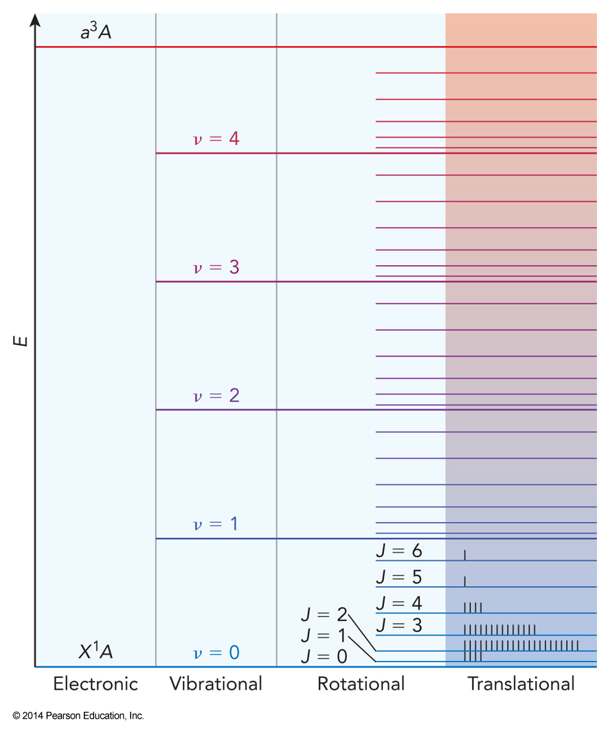
Equipartition Energy and Degrees of Freedom
Excitations
Example 3.1
From the equipartition principle, estimate the energies in \(\mathrm{J}\) that must be carried away to cool (a) \(0.500\,\chem{mol\, He(g)}\) and (b) \(0.500\, \chem{mol\, CO(g)}\) from \(1000\, \mathrm{K}\) to \(900\, \mathrm{K}\) at constant volume.
Vibrational and Rotational Partition Functions
Vibrational Partition Function
- For a single, non-degenerate, harmonic vibrational mode $$ q_\chem{vib}(T)=\sum_{v=0}^\infty e^{-\frac{v\omega_e}{k_\mathrm{B}T}} $$
- At very high temperatures or very low vibrational constants we can use the power series $$ q_\chem{vib}(T) = 1+e^{-\frac{\omega_e}{k_\mathrm{B}T}}+e^{-\frac{2\omega_e}{k_\mathrm{B}T}}+e^{-\frac{3\omega_e}{k_\mathrm{B}T}}+\dots $$
- Taylor series expansion $$ f(x)=\sum_{n=0}^\infty \frac{\left( x-x_0 \right)^n}{n!} \left. \left( \frac{d^n f(x)}{dx^n} \right) \right|_{x_0} $$
The Partition Function
- From this we get the partition function $$ q_\chem{vib}(T) = f\left( e^{-\frac{\omega_e}{k_\mathrm{B}T}} \right) = \frac{1}{1-e^{-\frac{\omega_e}{k_\mathrm{B}T}}} $$
- Polyatomic molecules have more than one vibrational mode so \( q_\chem{vib}(T) = q_\chem{vib}^{(\nu_1)}(T) q_\chem{vib}^{(\nu_2)}(T) \dots \)
- Degenerate modes must be treated as distinct motions in the product
Select Vibrational and Rotational Constants
| Molecule | \(\mu \\ (\chem{amu})\) | \(R_e \\ (\AA)\) | \(B \\ (\textrm{cm}^{-1})\) | \(\alpha_e \\ (\textrm{cm}^{-1})\) | \(D \\ (10^{-6}\, \textrm{cm}^{-1})\) | \(\omega_e \\ (\textrm{cm}^{-1})\) | \(\omega_ex_e \\ (\textrm{cm}^{-1})\) |
|---|---|---|---|---|---|---|---|
| \(\chem{{}^1H{}^1H}\) | 0.50 | 0.742 | 60.8536 | 3.062 | 46660 | 4401.21 | 121.34 |
| \(\chem{{}^1H{}^2D}\) | 0.67 | 0.742 | 45.6378 | 1.9500 | 3811.92 | 90.71 | |
| \(\chem{{}^2D{}^2D}\) | 1.01 | 0.742 | 30.442 | 1.0632 | 3118.46 | 117.91 | |
| \(\chem{{}^1H{}^{19}F}\) | 0.96 | 0.917 | 20.9557 | 0.798 | 2150 | 4138.32 | 89.88 |
| \(\chem{{}^1H{}^{35}Cl}\) | 0.98 | 1.275 | 10.5934 | 0.3702 | 532 | 2990.95 | 52.82 |
| \(\chem{{}^1H{}^{79}Br}\) | 1.00 | 1.414 | 8.3511 | 0.226 | 372 | 2649.67 | 45.21 |
| \(\chem{{}^1H{}^{127}I}\) | 1.00 | 1.609 | 3.2535 | 0.0608 | 526 | 2309.60 | 39.36 |
| \(\chem{{}^2D{}^{19}F}\) | 1.82 | 0.917 | 11.0000 | 0.2907 | 585 | 2998.19 | 45.76 |
| \(\chem{{}^{12}C{}^{16}O}\) | 6.86 | 1.128 | 1.9313 | 0.0175 | 6 | 2169.82 | 13.29 |
| \(\chem{{}^{14}N{}^{14}N}\) | 7.00 | 1.098 | 1.9987 | 0.0171 | 6 | 2358.07 | 14.19 |
| \(\chem{{}^{14}N{}^{16}O^+}\) | 7.47 | 1.063 | 1.9982 | 0.0190 | 2377.48 | 16.45 | |
| \(\chem{{}^{14}N{}^{16}O}\) | 7.47 | 1.151 | 1.7043 | 0.0173 | -37 | 1904.41 | 14.19 |
| \(\chem{{}^{14}N{}^{16}O^-}\) | 7.47 | 1.286 | 1.427 | 1372 | 8 |
More Select Vibrational and Rotational Constants
| Molecule | \(\mu \\ (\chem{amu})\) | \(R_e \\ (\AA)\) | \(B \\ (\textrm{cm}^{-1})\) | \(\alpha_e \\ (\textrm{cm}^{-1})\) | \(D \\ (10^{-6}\, \textrm{cm}^{-1})\) | \(\omega_e \\ (\textrm{cm}^{-1})\) | \(\omega_ex_e \\ (\textrm{cm}^{-1})\) |
|---|---|---|---|---|---|---|---|
| \(\chem{{}^{16}O{}^{16}O}\) | 8.00 | 1.207 | 1.4457 | 0.0158 | 5 | 1580.36 | 12.07 |
| \(\chem{{}^{19}F{}^{19}F}\) | 9.50 | 1.418 | 0.8828 | 891.2 | |||
| \(\chem{{}^{35}Cl{}^{35}Cl}\) | 17.48 | 1.988 | 0.2441 | 0.0017 | 0.2 | 560.50 | 2.90 |
| \(\chem{{}^{79}Br{}^{79}Br}\) | 39.46 | 2.67 | 0.0821 | 0.0003 | 0.02 | 325.29 | 1.07 |
| \(\chem{{}^{127}I{}^{79}Br}\) | 48.66 | 2.470 | 0.0559 | 0.0002 | 0.008 | 268.71 | 0.83 |
| \(\chem{{}^{127}I{}^{127}I}\) | 63.45 | 2.664 | 0.0374 | 0.0001 | -0.005 | 214.52 | 0.61 |
| \(\chem{{}^{23}Na{}^{23}Na}\) | 11.49 | 3.077 | 0.1548 | 0.0009 | 0.7 | 159.13 | 0.73 |
| \(\chem{{}^{133}Cs{}^{133}Cs}\) | 66.45 | 4.47 | 0.0127 | 0.00003 | 0.005 | 42.02 | 0.08 |
Example 3.2
Find the abundance of \(\chem{ICl}\) molecules in the ground and lowest excited vibrational states at \(300\,\mathrm{K}\), given that the vibrational constant \(\omega_e\) is \(384\,\mathrm{cm}^{-1}\).
Rotational Motion
- In the simplest case, the rotational energy of a linear molecule is approximated as \(E_\chem{rot}=BJ(J+1)\)
- Now we turn to evaluating $$ \mathcal{P}(J)=\frac{g_\chem{rot} e^{-\frac{E_\chem{rot}}{k_\mathrm{B}T}}}{q_\chem{rot}} $$
- Recall that \(g_\chem{rot}=2J+1\)
- When \(B \ll k_\mathrm{B}T\) $$ q_\chem{rot} = \sum_{J=0}^\infty g_\chem{rot} e^{-\frac{E_\chem{rot}}{k_\mathrm{B}T}} \approx \int_0^\infty g_\chem{rot} e^{-\frac{E_\chem{rot}}{k_\mathrm{B}T}} \, dJ $$
Simplification
$$ q_\chem{rot} = \sum_{J=0}^\infty g_\chem{rot} e^{-\frac{E_\chem{rot}}{k_\mathrm{B}T}} \approx \int_0^\infty g_\chem{rot} e^{-\frac{BJ(J+1)}{k_\mathrm{B}T}} \, dJ $$
- Further simplification yields $$ \begin{align} q_\chem{rot} \approx & \int_0^\infty g_\chem{rot} e^{-\frac{BJ(J+1)}{k_\mathrm{B}T}} \, d\left[ J(J+1) \right] = -\frac{k_\mathrm{B}T}{B} \left[ e^{-\frac{BJ(J+1)}{k_\mathrm{B}T}} \right]_0^\infty \\ &= \frac{k_\mathrm{B}T}{B} = \frac{\theta_\chem{rot}}{T} \end{align} $$
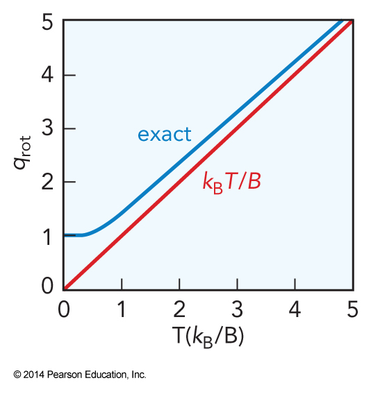
- This is called the integral approximation
The Integral Approximation To \(q_\chem{rot}\)
Combining Equations
- We can combine the vibrational and rotational probabilities $$ \begin{align} \mathcal{P}(v,J) &= \mathcal{P}_\chem{vib}(v) \mathcal{P}_\chem{rot}(J) = \left( \frac{g_\chem{vib} e^{-\frac{E_\chem{vib}}{k_\mathrm{B}T}}}{q_\chem{vib}(T)} \right) \left( \frac{g_\chem{rot} e^{-\frac{E_\chem{rot}}{k_\mathrm{B}T}}}{q_\chem{rot}(T)} \right) \\ &= \frac{g_\chem{vib} g_\chem{rot} e^{-\frac{E_\chem{vib}+E_\chem{rot}}{k_\mathrm{B}T}}}{q_\chem{vib}(T)q_\chem{rot}(T)} \end{align} $$
Example 3.3
Compare the rotational partition functions for \(\chem{CO}\) (\(\frac{B}{k_\mathrm{B}} = 2.70\,\mathrm{K}\)) obtained by using the integral and by using the direct sum, at \(273\,\mathrm{K}\) and at \(10\,\mathrm{K}\).
Example 3.4
Find the number density of \(\chem{OCS}\) molecules in a \(100.0\,\mathrm{Pa}\) sample at \(298\,\mathrm{K}\) that are in the vibrational state \((v_1, v_2, v_3) = (1, 0, 1)\) and rotational state \(J = 10\). The constants of \(\chem{CS}\)-stretch \(\omega_1 = 859\,\mathrm{cm}^{-1}\), bend \(\omega_2 = 527\,\mathrm{cm}^{-1}\), and \(\chem{CO}\)-stretch \(\omega_3 = 2080\,\mathrm{cm}^{-1}\), \(B = 0.2028\,\mathrm{cm}^{-1}\). The bending mode is a doubly degenerate vibrational motion, so it counts for two modes. Give the final value in molecules per cubic centimeter.
Another Rotational Partition Function
- The rotational partition function of non-linear molecules are evaluated in terms of three rotational constants, \(A\), \(B\), and \(C\) $$ q_\chem{rot(nonlinear)} \approx \left( \frac{\pi k_\mathrm{B}^3 T^3}{ABC} \right)^\bfrac{1}{2} $$
- Works best for symmetric tops \(A=B\) (oblate) or \(B=C\) (prolate)
- Still useful for asymmetric tops \(A \ne B \ne C\)
Complications of Rotations
- Molecules with proper rotation axes, \(q_\chem{rot}\) depends on the molecule’s nuclear spin, ns, statistics
- Many molecules have atoms that are exactly identical, called equivalent atoms
- If a rotation exchanges equivalent atoms, we need to worry about the symmetrization principle
- We can write the total wavefunction as $$ \Psi_\chem{total} = \psi_\chem{elec} \psi_\chem{vib} \psi_\chem{rot} \psi_\chem{ns} $$
Example: \(\chem{{}^1H_2}\)
- There are two spin possibilities \(+\frac{1}{2}\) (\(\alpha\)) or \(-\frac{1}{2}\) (\(\beta\))
- Total nuclear spin: \( \left| I_T \right| = \left| \vec{I}_A + \vec{I}_B \right| = 0\text{ or }1 \)
- \(\left| I_T \right|=1\) is symmetric to permutation operator
- \(\left| I_T \right|=0\) is antisymmetric to permutation operator
- \(\chem{{}^1H}\) nuclei are fermion and therefore must be antisymmetric to exchange overall
- This requirement gives rise to two sets of states, three triplet states and one singlet state
Nuclear Spin States
- The singlet state mathematically is $$ \psi_\chem{ns} = \frac{1}{\sqrt{2}} \left[ \alpha(A)\beta(B) - \beta(A)\alpha(B) \right]\;\text{note: }I_T=0 $$
- The triplet set mathematically are, \(I_T = 1\) $$ \psi_\chem{ns} = \begin{cases} \alpha(A)\alpha(B) \\ \frac{1}{\sqrt{2}} \left[ \alpha(A)\beta{B} + \beta{A}\alpha{B} \right] \\ \beta(A)\beta(B) \end{cases} $$
Symmetric vs Antisymmetric
- The singlet state is antisymmetric to exchange
- The triplet states are symmetric to exchange
- The overall wavefunction must be antisymmetric
- Now we have to check the symmetries of the other degrees of freedom
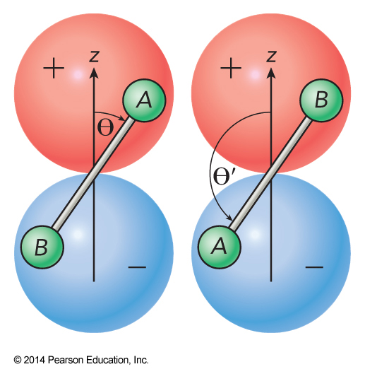
- Consider rotational wavefunctions for \(J = 1\) and \(2\), \(M_J = 0\) $$ \begin{align} Y_1^0 (\Theta) &= \cos \Theta \\ Y_2^0(\Theta) &= \left( 3\cos^2 \Theta - 1 \right) \end{align} $$
Exchange Symmetry of Rotations
- Exchanging the labels, reverses the direction $$ \Theta' = \pi - \Theta $$
- This means
- \(\cos \Theta\) changes sign
- \(\cos^2\Theta\) does not change sign
Overall Rotational Symmetry
- From this analysis we know that:
- Odd J states are antisymmetric with respect to exchange
- Even J states are symmetric with respect to exchange
- For the \( {}^1\Sigma_g^+ \) ground state \(\chem{H_2}\), the electronic wavefunction is totally symmetric
- For a diatomic molecule, the vibrational wavefunction is always totally symmetric
Meaning
- What we now know is that for \(\chem{{}^1H_2}\):
- The singlet nuclear spin state (antisymmetric) may occupy only even \(J\) states (symmetric)
- The triplet nuclear spin state (symmetric) may occupy only the odd \(J\) states (antisymmetric)
- The degeneracy of the rotational state now depends on the nuclear spins
- Note: \(g\) electronic and vibrational wavefunctions are symmetric and \(u\) are antisymmetric
Spin Statistics Effects on the Partition Function
- We found that the triplet state has an added factor of three in its degeneracy of \(\chem{{}^1H_2}\)
- Different nuclear spin states of a molecule act almost independently of each other
- They are best described by separate partition functions
- Energies are referenced to the lowest energy of the particular spin state
Rotational Partition Function for \(\chem{{}^1H_2}\)
$$ \begin{align} q_\chem{rot}\left(\chem{H_2}\right) =& q_\chem{rot}\left(I_T=0\right) + q_\chem{rot}\left(I_T=1\right) \\ =& \left[ 1+5e^{-\frac{6B}{k_\mathrm{B}T}}+9e^{-\frac{20B}{k_\mathrm{B}T}}+\dots \right] \\ & +3 \left[ 3e^{-\frac{(2-2)B}{k_\mathrm{B}T}}+7e^{-\frac{(12-2)B}{k_\mathrm{B}T}}+11e^{-\frac{(30-2)B}{k_\mathrm{B}T}}+\dots \right] \end{align} $$
- This is a dramatic effect in hydrogen
- Para-hydrogen – \(I_T = 0\)
- Ortho-hydrogen – \(I_T = 1\)
Other Systems
- For homonuclear boson diatomics, such as \(\chem{O_2}\), or other symmetric linear systems, such as \(\chem{CO_2}\), the overall wavefunction must be symmetric
- As a general (approximate) rule, rotational partition functions in molecules where rotation exchanges \(n\) equivalent \(I = 0\) nuclei will be reduced by a factor of \(\frac{1}{n}\).
The Translational Partition Function
Translations
- The quantum energies of translational energies $$ \varepsilon = n^2 \frac{h^2}{8mV^\bfrac{2}{3}} = n^2 \varepsilon_0 $$
- Molecules are rarely confined to small enough volumes for the energies levels to become important
- The classical limit is an approximation of a degree of freedom that remains quantum mechanical
Counting the Energy Levels
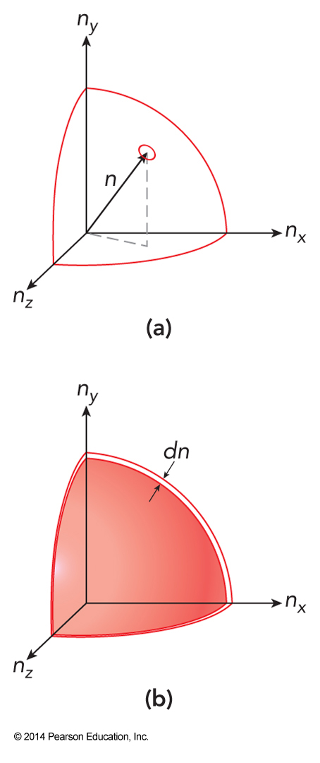
- How many values of \(n_x\), \(n_y\), and \(n_z\) that give the same value of \(n^2\) (proportional of \(\varepsilon\))? $$ n\equiv \sqrt{n^2} = \left( n_x^2 + n_y^2+n_z^2 \right)^\bfrac{1}{2} $$
- The degeneracy is roughly the number of distinct points in a shell of width \(dn\) that lies between a radius of \(\sqrt{n^2}\) and \(\sqrt{n^2+1}\)
The Integral Approximation To \(q_\chem{rot}\)
Counting Points on a Surface
The Number of Points
- We can estimate the \(dn\) by $$ \begin{align} d\left( n^2 \right) &= 2n\,dn =1 \\ dn &= \frac{1}{2n} \end{align} $$
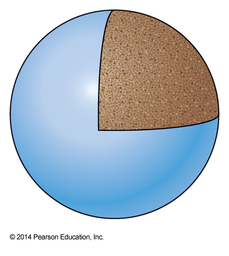
- The degeneracy is the same as the ensemble size \(\Omega\) for the system at this energy $$ \Omega = \frac{4\pi n^2}{8}dn = \frac{\pi}{2}n^2\,dn = \frac{\pi}{2}n^2\frac{1}{2n} = \frac{\pi}{4}n = \frac{\pi}{4}\left(\frac{\varepsilon}{\varepsilon_0}\right)^\bfrac{1}{2} $$
Density of States
- Now we can find the density of quantum states, \(W\) $$ W(\varepsilon) = \frac{\Omega}{\varepsilon_0} = \frac{\pi}{4\varepsilon_0^\bfrac{3}{2}} \varepsilon^\bfrac{1}{2} $$
- Now we can build the partition function
- Due to the involved derivation, here’s the results $$ q_\chem{trans}(T,V) = q'_K(T) q'_U(T,V)=\underbrace{\left(\frac{2 \pi m k_\mathrm{B}T}{h^2}\right)^\bfrac{3}{2}}_{q'_K(T)} \underbrace{V}_{q'_U(T,V)} $$
Temperature and the Maxwell-Boltzmann Distribution
The Energies
- At low energy, energy can only be stored as translational degrees of freedom so that $$ E=\sum_{j=1}^N \left( \frac{1}{2} mv_j^2 \right) = \frac{1}{2}mN\expect{v^2} $$
- Rewritten $$ E=\frac{1}{2}mN\expect{v_x^2+v_y^2+v_z^2} = \frac{3}{2}mN\expect{v_x^2} $$
- Remember previous equations $$ \expect{x^2} = \frac{k_\mathrm{B}T}{2a} \therefore E=\frac{3}{2}mN\left( \frac{k_\mathrm{B}T}{m} \right) = \frac{3}{2}Nk_\mathrm{B}T = \frac{3}{2}nRT $$
Example 3.5
Calculate the root mean square momentum along the \(x\) axis \(\expect{p_x^2}^\bfrac{1}{2}\) in \(\mathrm{kg\, m\, s^{-1}}\) of a helium atom in the gas-phase when the temperature is \(312\, \mathrm{K}\). (We don’t want to calculate \(\expect{p_x}\) because that should average to zero, motion in the \(+x\) and \(–x\) directions being equally likely.)
Questions
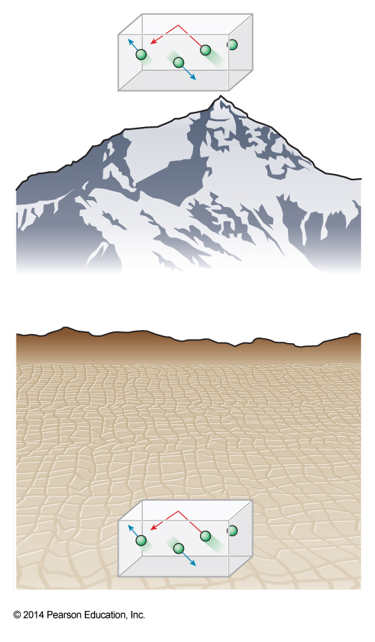
- Why does \(T\) depend on only the easily excited degrees of freedom?
- Degree of freedom that isn’t excited doesn’t contribute to the degeneracy of quantum states.
- Why does \(T\) depend on only the kinetic energy?
- Once we have established the confines of the system and the forces, the potential energy becomes a fixed parameter and the kinetic energy can adjust to change the degeneracy.
Easily Excited Degrees of Freedom
Temperature and Kinetic Energy
Boltzmann Constant and Temperature
- The Boltzmann constant is just a conversion factor between temperature and kinetic energy $$ \frac{E}{N} = \expect{\varepsilon} = \frac{3k_\mathrm{B}T}{2} $$
- Temperature is an intensive parameter, like pressure
Example 3.6
Find the average translational kinetic energy (in \(\mathrm{kJ\, mol^{-1}}\)) and the rms speed along the \(x\) axis \(\expect{v_x^2}^\bfrac{1}{2}\) for a nitrogen molecule at \(298\, \mathrm{K}\).
The Probability Distribution
- We can now work on the probability distribution $$ \begin{align} \mathcal{P}_\vec{v}(\vec{v}) &= \frac{e^{-\frac{mv^2}{2k_\mathrm{B}T}}}{\int_{-\infty}^\infty \int_{-\infty}^\infty \int_{-\infty}^\infty e^{-\frac{mv^2}{2k_\mathrm{B}T}} \, dv_x\,dv_y\,dv_z} \\ &= \frac{e^{-\frac{mv^2}{2k_\mathrm{B}T}}}{\frac{h^3 q'_K(T)}{m^3}} \\ &= \left( \frac{m}{2\pi k_\mathrm{B}T} \right)^\bfrac{3}{2} e^{-\frac{mv^2}{2k_\mathrm{B}T}} \end{align} $$
Moving to Speed Instead of Velocity
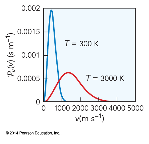
- We can integrate away the directions to get to speed instead of velocity $$ \begin{align} \mathcal{P}_v(v) &= \int_0^{2\pi} \int_0^\pi \mathcal{P}_\vec{v}(\vec{v}) v^2\, dv\, \sin \Theta\, d\Theta\, d\Phi \\ &= 4\pi \mathcal{P}_\vec{v}(\vec{v}) v^2\,dv \\ \mathcal{P}_v(v) &= 4\pi \left( \frac{m}{2\pi k_\mathrm{B}T} \right)^\bfrac{3}{2} v^2 e^{-\frac{mv^2}{2k_\mathrm{B}T}} \end{align} $$
Exchange Symmetry of RotationsQuantizer Energy
- Little population at the lowest speeds
- Little population at the highest speeds
- As temperature increases, the distribution shifts towards higher \(E\)
Example 3.7
In a \(1.00\, \mathrm{mole}\) sample of \(\chem{N_2}\) at \(298\, \mathrm{K}\), calculate the number of molecules that will have speeds \(v\) within \(0.005\, \mathrm{m\, s^{-1}}\) of \(10.0\, \mathrm{m\, s^{-1}}\).
Maxwell-Boltzmann Distribution: Average Velocity
$$ \begin{align} \expect{v} &= \frac{\int_0^\infty \mathcal{P}_v(v) v\,dv}{\int_0^\infty \mathcal{P}_v(v)\,dv} \\ &= \frac{4\pi \int_0^\infty e^{-\frac{mv^2}{2k_\mathrm{B}T}} v^3 \,dv}{4\pi \int_0^\infty e^{-\frac{mv^2}{2k_\mathrm{B}T}} v^2 \,dv} \\ &= \frac{\frac{1}{2}\left( \frac{2k_\mathrm{B}T}{m} \right)^2}{\frac{1}{4}\left( \frac{2\pi k_\mathrm{B}^3T^3}{m^3} \right)^\bfrac{1}{2}} \\ &= \left( \frac{8k_\mathrm{B}T}{\pi m} \right)^\bfrac{1}{2} = \sqrt{\frac{8k_\mathrm{B}T}{\pi m}} \end{align} $$
/